4 环境数据统计分析

数学分析是从公理体系出发，采用演绎法将普适规律应用于特殊领域(从一般到个别)，而统计分析是从实际观测数据出发，采用归纳法从特殊现象总结出普适规律(从个别到一般)。与数学分析方法一样，统计分析方法也是一种重要的科学研究方法，普遍应用于自然科学、社会科学、经济学等诸多领域。

尽管环境数据规模和维度越来越大，统计分析仍然是探索和分析此类大数据的有效手段，同时也是机器学习的基础。常用的数据统计分析方法包括描述性统计(descriptive statistics)、推断性统计(inferential statistics)、相关分析(correlation analysis)、回归分析(regression analysis)、主成分分析(principal component analysis，PCA)、因子分析(factor analysis，FA)、聚类分析(clustering analysis)等。

本章基于R语言介绍描述性统计分析、推断性统计分析、相关分析、回归分析、主成分分析、因子分析以及聚类分析。

4.1 描述性统计

描述性统计分析是以一种简单而有意义的方式来描述、显示和概括原始数据，亦可称之为探索性数据分析(Exploratory Data Analysis，EDA)，主要包括频数分析、集中趋势分析、离散程度分析、数据分布特征以及一些基本的统计图表。

4.1.1 频数分析

频数分析是按某个分类变量分组或按某个数值变量分区间对数据进行频数统计，以了解数据在这些有意义的组或区间上的具体分布。在频数的基础上，可以进一步计算频率、累积频率等指标。直方图是最常用的频数分析的可视化方式。R提供的table()函数可对数据集中某个分类变量进行频数统计(结果为频数分布表，也称为一维列联表)，xtabs()函数根据两个分类变量创建交叉频数统计(结果为二维列联表)，prop.table()函数在频数统计的结果上计算频率，addmargins()函数为频数或频率统计结果计算行列之和。在R Markdown和Quarto文档中，可利用knitr包中的kable()函数美化频数统计表的输出。

例 4.1 下面是一个对河流水质数据进行的频数分析。

library(tidyverse)

set.seed(2022)
#随机构造数据：rn为河流名称，wq为水质等级，wt为河流类型
data <- tibble(
  rn = paste("河流", 1:50),
  wq = sample(c("I类","II类","III类","IV类","V类","劣V类"),
              50, replace = TRUE),
  wt = sample(c("小型河流","中型河流","大型河流"),
              50, replace = TRUE)) %>% 
  mutate(wq = factor(wq,levels = c("I类","II类","III类",
                                   "IV类","V类","劣V类"),
                 ordered = TRUE),
         wt = factor(wt,levels = c("小型河流","中型河流",
                                   "大型河流"),
                 ordered = TRUE))
data

# A tibble: 50 × 3
   rn      wq    wt      
   <chr>   <ord> <ord>   
 1 河流 1  IV类  大型河流
 2 河流 2  III类 中型河流
 3 河流 3  劣V类 小型河流
 4 河流 4  III类 大型河流
 5 河流 5  IV类  中型河流
 6 河流 6  劣V类 中型河流
 7 河流 7  劣V类 大型河流
 8 河流 8  IV类  大型河流
 9 河流 9  III类 大型河流
10 河流 10 I类   小型河流
# ℹ 40 more rows

t1 <- data$wq %>% table() 
t1 %>% knitr::kable()

.	Freq
I类	7
II类	7
III类	10
IV类	10
V类	7
劣V类	9

t2 <- data %>% xtabs(~ wq + wt, .)
t2 %>% knitr::kable()

	小型河流	中型河流	大型河流
I类	4	2	1
II类	1	3	3
III类	2	4	4
IV类	3	3	4
V类	3	1	3
劣V类	2	3	4

t2 %>% 
  addmargins() %>% 
  knitr::kable()

	小型河流	中型河流	大型河流	Sum
I类	4	2	1	7
II类	1	3	3	7
III类	2	4	4	10
IV类	3	3	4	10
V类	3	1	3	7
劣V类	2	3	4	9
Sum	15	16	19	50

t2 %>% 
  prop.table() %>% 
  addmargins() %>% 
  knitr::kable()

	小型河流	中型河流	大型河流	Sum
I类	0.08	0.04	0.02	0.14
II类	0.02	0.06	0.06	0.14
III类	0.04	0.08	0.08	0.20
IV类	0.06	0.06	0.08	0.20
V类	0.06	0.02	0.06	0.14
劣V类	0.04	0.06	0.08	0.18
Sum	0.30	0.32	0.38	1.00

cumsum()函数用于计算累积频数或频率：

df <- t1 %>% 
  prop.table() %>% 
  as.data.frame() %>% 
  mutate(CumFreq = cumsum(Freq))
df

      . Freq CumFreq
1   I类 0.14    0.14
2  II类 0.14    0.28
3 III类 0.20    0.48
4  IV类 0.20    0.68
5   V类 0.14    0.82
6 劣V类 0.18    1.00

频数分布表可以用as.data.frmae()函数转换为数据框类型。

对数值变量做分组频数统计，需要先确定分组区间界值及相应的标签，再用cut()函数根据区间界值对数据分组，然后用table()和prop.table()函数进行频数和频率统计。

例 4.2 现有某市2014年冬季(2014年12月-2015年2月)的每日AQI指数，共90个数据(如下表所示)，对其做频数分析。

月份	AQI
12月	86 62 75 71 78 107 130 137 86 119 134 81 76 92 132 70 55 79 79 108 78 71 99 150 117 65 95 105 103 94 73
1月	64 79 94 310 194 185 91 98 99 165 142 97 76 72 86 183 161 127 98 99 199 141 154 185 257 264 118 53 56 142 135
2月	67 99 147 217 121 80 103 72 62 70 95 120 240 164 74 196 212 139 77 42 55 130 132 96 70 144 54 29

根据《环境空气质量评价技术规范(试行)》(HJ 663—2013)的规定，AQI(空气质量指数)分级如下：0~50为优(一级)，51~100为良(二级)，101~150为轻度污染(三级)，151~200为中度污染(四级)，201~300为重度污染(五级)，>300为严重污染(六级)。先通过电子表格软件如WPS表格或Office Excel，输入数据，第一列列名为Month，第二列列名为Day，第三列列名为AQI，最后命名保存为aqi-data.csv数据文件。

library(tidyverse)

df <- read_csv("./data/aqi-data.csv")
labels <- c("优", "良", "轻度污染", "中度污染", "重度污染", "严重污染")
breaks <- c(0, 51, 101, 151, 201, 301, Inf)
aqi <- cut(df$AQI, breaks = breaks, labels = labels,
           include.lowest = TRUE)
# include.lowest参数为TRUE时表示区间包含界值下限，为FALSE时表示包含界值上限
ft <- as.data.frame(table(Group = aqi))
library(dplyr)
dft <- ft %>% 
  mutate(CumFreq = cumsum(Freq),
         FreqRate = prop.table(Freq)) %>% 
  mutate(CumFreqRate = cumsum(FreqRate)) %>% 
  mutate(FreqRate = round(FreqRate * 100, 2),
         CumFreqRate = round(CumFreqRate * 100, 2))
dft

     Group Freq CumFreq FreqRate CumFreqRate
1       优    2       2     2.22        2.22
2       良   47      49    52.22       54.44
3 轻度污染   25      74    27.78       82.22
4 中度污染   10      84    11.11       93.33
5 重度污染    5      89     5.56       98.89
6 严重污染    1      90     1.11      100.00

由以上频数分析结果可见，该城市冬季AQI为“优”和“良”的累积比例超过54%。

dft$Group <- ordered(dft$Group,                     
                     levels = c("优","良","轻度污染","中度污染",
                                "重度污染","严重污"))
ggplot(dft, aes(x = Group, y = Freq)) + 
  geom_col() +   
  geom_text(aes(label = Freq), vjust = -0.5) +  
  ylim(c(0,55)) +   
  labs(x = "空气质量等级", y = "累计天数") +  
  theme_bw()

在除尘系统设计中，也需要对颗粒物粒径进行类似的频数统计，从而更好地了解尘粒的粒径分布以计算分级除尘效率。

4.1.2 集中趋势

集中趋势反映一组变量值的集中位置，用于描述数据的一般水平。集中趋势用平均数表示，包括算术平均数、几何平均数、调和平均数、中位数、百分位数和众数，前三者为数值平均数，后三者为位置平均数。数值平均数综合了所有数据，受极值影响较大，且不适用于定类和定序数据；位置平均数不受极值的影响，适用于定序数据。要注意，众数不具有唯一性，有时无法计算得到，只有对大量数据计算众数才有意义。

计算数值平均数的方法：

计算算术平均数: mean()。
计算加权算术平均数: weighted.mean()。
计算几何平均数: psych::geometric.mean()，或pracma::geomean()，或exp(mean(log(x)))。几何平均数受极值的影响较算术平均数小，适用于等比或近似等比关系的数据，计算时要注意负数的影响。
计算调和平均数(倒数的算术平均数的倒数)：psych::harmonic.mean()，或pracma::harmmean()。调和平均数实际应用范围较小，一般用于因缺乏总体单位数而不能直接计算算术平均数的场合，计算时要注意0值的影响。

对于同一组数据，调和平均数≤几何平均数≤算术平均数。

计算位置平均数的方法：

中位数: median()。中位数是数据排序后居于中间位置的数值，不受两端极值影响，在非正态分布数据中较算术平均数更有代表性。
百分位数: quantile()。百分位数是中位数的扩展，有些数据需要了解其1%、5%、10%、25%、75%、90%、95%、99%、99.99%等位置上的数值，如环境毒理学研究、除尘技术研发等；其中居于25%和75%位置上的数据分别称为下四分位数(Q1)和上四分位数(Q3)。
众数: 众数是数据集中出现频次最高的数值。计算众数首先要排除无法计算的情况(如所有数值出现的频数相等)，然后先计算频数：tbl = as.data.frame(table(x))，再找出最大频数：max_freq = max(tbl[ , 2])，最后找出最大频数对应的数值：mode = tbl[tbl[ , 2] == max_freq, 1]

通过算术平均数、中位数以及众数的关系可以判断数据的大致分布类型(如图 4.2 所示)：对于理想的对称分布，算术平均数 = 中位数 = 众数；在右偏分布的资料中，算术平均数＞中位数＞众数；在左偏分布的资料中，算术平均数＜中位数＜众数。

例 4.3 计算数值平均数。

# 算术平均数
# 计算废水中铬浓度10次测定结果的算术平均数
cr_conc <- c(0.92, 0.83, 0.82, 0.91, 1.06, 0.88, 1.07, 0.84, 1.01, 0.96)
mean(cr_conc)

[1] 0.93

# 分组频数资料加权计算算术平均数
so2_conc <- c(0.44, 0.48, 0.52, 0.56, 0.60)    # 二氧化硫分组组中值
f <- c(3, 5, 9, 3, 5)    # 对应频数
wm <- weighted.mean(so2_conc, f)
round(wm, 2)

[1] 0.52

# 几何平均数
# 8个样本中某污物染浓度测定值(近似等比资料)
p_conc <- c(10, 10, 20, 20, 40, 80, 160, 326)
# 利用对数法计算
logpc <- log10(p_conc)
n <- length(p_conc)
gm <- 10^(sum(logpc) / n)    # 对数法
round(gm, 2)

[1] 40.09

# 利用psych包计算
round(psych::geometric.mean(p_conc), 2)

[1] 40.09

# 调和平均数
# 4个化工园区废水处理量和处理率，求平均处理率
wv  <- c(30000, 50000, 25000, 18000)    # 废水处理量
pt <- c(65, 75, 95, 55)    # 废水处理率
hm <- sum(wv) / sum(wv / (pt / 100))
round(hm * 100, 2)

[1] 71.57

例 4.4 计算位置平均数。

# 中位数
# 10个废水BOD浓度测定值
bod <- c(50, 53.5, 51, 53.5, 52, 55, 58, 53, 56, 53.5)
median(bod)

[1] 53.5

# 计算1%、5%、95% 99%分位数
# 随机生成颗粒物粒径数据(利用对数正态分布函数)
set.seed(2022)
p_size <- rlnorm(1000, meanlog = 3, sdlog = 1)
qp <- quantile(p_size, probs = c(0.01, 0.05, 0.95, 0.99))
round(qp, 2)

    1%     5%    95%    99% 
  2.16   4.23  99.19 232.50

# 计算众数
set.seed(2022)
bod <- c(50, 53.5, 51, 53.5, 52, 55, 58, 53, 56, 53.5)
tbl <- as.data.frame(table(bod))    # 统计频数并转换成数据框类型
max_freq <- max(tbl[ , 2])    # 找到最大的频数
tbl[tbl[ , 2] == max_freq, 1]    # 频数最大的数值即众数

[1] 53.5
Levels: 50 51 52 53 53.5 55 56 58

计算总和可用sum()函数，对于矩阵还可用rowSums()、colSums()、rowMeans()和colMeans()分别求其行和列的和与算术平均数，也可利用apply()函数与sum()或mean()结合来计算行与列的和或算术平均数。

例 4.5 计算矩阵行列总和与平均数。

mat <- matrix(1:24, nrow = 4, byrow = TRUE)
mat

     [,1] [,2] [,3] [,4] [,5] [,6]
[1,]    1    2    3    4    5    6
[2,]    7    8    9   10   11   12
[3,]   13   14   15   16   17   18
[4,]   19   20   21   22   23   24

rowSums(mat)

[1]  21  57  93 129

colSums(mat)

[1] 40 44 48 52 56 60

rowMeans(mat)

[1]  3.5  9.5 15.5 21.5

colMeans(mat)

[1] 10 11 12 13 14 15

apply(mat, 1, sum)

[1]  21  57  93 129

apply(mat, 2, sum)

[1] 40 44 48 52 56 60

4.1.3 离散程度

离散程度反映数据偏离中心位置的程度，用于描述数据的变异大小。离散程度用变异数表征，变异指标包括极差(亦称全距，range)、四分位间距(interquartile range，IQR)、标准差(standard deviation，SD)、方差(variance，VAR)、标准误(standard error，SE)以及变异系数(coefficient of variation，CV)，其中方差和标准差最为常用。

极差: max(x) – min(x)，即为数据中最大值与最小值之差。仅使用了数据中两个极端观测值，稳定性差。
四分位间距: IQR(x)，即上、下四分位数之差。与极差相比，IQR不受极值影响，具有较好的稳定性，但仍然只使用了数据集中2个观测值。
方差: 总体方差用sum((x - mean(x))^2) / length(x)计算，样本方差用var(x)计算。方差综合考虑了数据中所有观测值的变异，是更有代表性也被经常使用的离散程度指标。
标准差: 由于方差的量纲与原数据不同，故引入标准差，即方差的平方根。总体标准差用sqrt()计算总体方差的平方根，样本标准差直接用sd()计算。
标准误: sd(x) / sqrt(length(x))，即样本均值的标准误差，用于衡量样本均值和总体均值的偏差大小。
变异系数: 相对变异指标，消除了量纲和平均数差异的影响，便于比较不同组数据之间的离散程度。常用的变异系数为标准差变异系数，计算方法为sd(x) / abs(mean(x)) * 100，或直接使用raster::cv()函数。

例 4.6 计算各种变异指标。

library(readr)

# 读入aqi数据
df <- read_csv("./data/aqi-data.csv")
x <- df$AQI

# 计算极差
max(x) - min(x)

[1] 281

# 计算四分位间距
IQR(x)

[1] 62.5

# 计算样本方差
var(x)

[1] 2821.243

# 计算样本标准差
sd(x)

[1] 53.11537

# 计算标准误
sd(x) / sqrt(length(x))

[1] 5.598852

# 计算变异系数
raster::cv(x)

[1] 46.69255

sd(x) / abs(mean(x)) * 100

[1] 46.69255

4.1.4 数据分布特征

环境数据的统计分析，通常需要对样本的分布做出假设，绝大多数的统计分析方法要求样本分布(近似)为正态分布。样本的分布特征可以用偏度(skewness)和峰度(kurtosis)来描述。

偏度用于描述数据分布偏斜方向和程度，如果是对称分布(如图 4.2 中图所示)，则偏度为0；如果是左偏分布(亦称负偏态，分布高峰偏右，如图 4.2 左图所示)，偏度为负值；如果是右偏分布(亦称正偏态，分布高峰偏左，如图 4.2 右图所示)，偏度为正值。

峰度用于表征概率密度曲线在平均值处的峰值高低，也反映了尾部的厚度。当数据分布接近正态分布时，峰度接近于0；当数据分布两侧的极端数据更多时，峰度为负值；当数据分布两侧的极端数据更少时，峰度为正值。

有很多R包提供了计算偏度和峰度的函数，此处介绍e1071包中偏度和峰度的计算函数skewness()和kurtosis()。e1071包中偏度和峰度的计算均有三个不同的公式，在函数中以type参数指定，参数值为1、2和3，默认type=3。在资料为正态分布时，这三个公式计算的偏度都是无偏估计值，而峰度只有第二个公式的计算结果为无偏估计值。psych包中计算偏度和峰度函数为skew()和kurtosi()，与e1071包的计算方法一致。

例 4.7 计算偏度和峰度。

df <- read_csv("./data/aqi-data.csv")
x <- df$AQI

e1071::skewness(x, type = 1)

[1] 1.312296

e1071::skewness(x, type = 2)

[1] 1.334644

e1071::skewness(x, type = 3)

[1] 1.290485

e1071::kurtosis(x, type = 1)

[1] 1.765053

e1071::kurtosis(x, type = 2)

[1] 1.936933

e1071::kurtosis(x, type = 3)

[1] 1.659751

# 生成1000个正态数据(样本均值为0，标准差为1)
set.seed(2022)
y <- rnorm(1000)
skewness(y)

[1] 0.07010706

kurtosis(y)

[1] 0.08095659

从例 4.7 的计算结果可以发现，标准正态分布数据的偏度和峰度均接近于0。

Q-Q图(x轴为理论分位数，y轴为样本数据分位数；符合正态分布时，二者应呈直线关系)和经验分布函数图(比较样本经验分布和理论分布曲线的重合程度)可用来直观地判断数据分布是否符合或近似正态分布。R中qqnorm()和qqline()函数分别用于绘制Q-Q图及其相应直线，ecdf()函数用于计算样本数据的经验分布，再通过plot()绘制出图形，与理论分布函数曲线(pnorm()函数计算理论概率并用lines()函数绘制曲线)进行比较。

例 4.8 绘制例 4.7 中x和y的Q-Q图(结果如图 4.3 所示)。

# 偏态数据
df <- read_csv("./data/aqi-data.csv")
x <- df$AQI
qqnorm(x)
qqline(x, col = "red")

# 正态数据
set.seed(2022)
y <- rnorm(100)
qqnorm(y)
qqline(y, col = "red")

library(ggplot2)
ggplot(df, aes(sample = AQI)) + 
  geom_qq(size = 0.6) +
  geom_qq_line(color = "red") +
  theme_bw()

set.seed(2022)
dfn <- data.frame(
  val = rnorm(100)
)
ggplot(dfn, aes(sample = val)) + 
  geom_qq(size = 0.6) +
  geom_qq_line(color = "red") +
  theme_bw()

由图 4.3 可见，AQI数据的分位数与正态分布的理论分位数在两端的差异非常明显，表明其分布不符合正态分布；而构造的标准正态数据的样本分位数与理论分位数呈明显的直线关系，表明其符合正态分布。

例 4.9 绘制经验累积分布函数曲线图与理论累积分布函数曲线(结果如图 4.4 所示，其中红色平滑曲线为理论累积分布密度函数曲线，蓝色为经验累积分布密度函数曲线，即数据实际的累积分布密度)。

# 偏态数据
df <- read_csv("./data/aqi-data.csv")
x <- df$AQI
plot(ecdf(x), verticals = TRUE, do.p = FALSE, col = "blue")
m <- c(min(x):max(x))
lines(m, pnorm(m, mean(x), sd(x)), col = "red")    # 理论分布

# 正态数据
set.seed(2022)
y <- round(rnorm(100, 20, 5))
plot(ecdf(y), verticals = TRUE, do.p = FALSE, col = "blue")
m <- c(min(y):max(y))
lines(m, pnorm(m, mean(y), sd(y)), col = "red")    # 理论分布

由图 4.4 (b) 可见，根据正态分布生成的数据的样本经验分布函数与理论分布函数的曲线基本重合。

4.1.5 数据摘要

R中summary()函数可以提供数据的基本摘要信息，对数值变量，可显示其最小值、最大值、算术平均数、中位数、Q1和Q3以及缺失数。与之相比，psych包提供的describe()函数提供的摘要信息更为全面，对数值变量，除了summary()函数提供的信息外，还包括截断均值、标准差、标准误、极差、四分位间距、绝对中位数偏差、偏度和峰度等信息。skimr包提供的skim()函数强化了对缺失数据的分析，并对数值变量给出频数分布直方图。

例 4.10 比较summary()、describe()和skim()三个数据摘要函数的差异。

summary(airquality)

     Ozone           Solar.R           Wind             Temp      
 Min.   :  1.00   Min.   :  7.0   Min.   : 1.700   Min.   :56.00  
 1st Qu.: 18.00   1st Qu.:115.8   1st Qu.: 7.400   1st Qu.:72.00  
 Median : 31.50   Median :205.0   Median : 9.700   Median :79.00  
 Mean   : 42.13   Mean   :185.9   Mean   : 9.958   Mean   :77.88  
 3rd Qu.: 63.25   3rd Qu.:258.8   3rd Qu.:11.500   3rd Qu.:85.00  
 Max.   :168.00   Max.   :334.0   Max.   :20.700   Max.   :97.00  
 NA's   :37       NA's   :7                                       
     Month            Day      
 Min.   :5.000   Min.   : 1.0  
 1st Qu.:6.000   1st Qu.: 8.0  
 Median :7.000   Median :16.0  
 Mean   :6.993   Mean   :15.8  
 3rd Qu.:8.000   3rd Qu.:23.0  
 Max.   :9.000   Max.   :31.0

psych::describe(airquality, IQR = TRUE, quant = c(0.25, 0.75))

        vars   n   mean    sd median trimmed   mad  min   max range  skew
Ozone      1 116  42.13 32.99   31.5   37.80 25.95  1.0 168.0   167  1.21
Solar.R    2 146 185.93 90.06  205.0  190.34 98.59  7.0 334.0   327 -0.42
Wind       3 153   9.96  3.52    9.7    9.87  3.41  1.7  20.7    19  0.34
Temp       4 153  77.88  9.47   79.0   78.28  8.90 56.0  97.0    41 -0.37
Month      5 153   6.99  1.42    7.0    6.99  1.48  5.0   9.0     4  0.00
Day        6 153  15.80  8.86   16.0   15.80 11.86  1.0  31.0    30  0.00
        kurtosis   se    IQR  Q0.25  Q0.75
Ozone       1.11 3.06  45.25  18.00  63.25
Solar.R    -1.00 7.45 143.00 115.75 258.75
Wind        0.03 0.28   4.10   7.40  11.50
Temp       -0.46 0.77  13.00  72.00  85.00
Month      -1.32 0.11   2.00   6.00   8.00
Day        -1.22 0.72  15.00   8.00  23.00

skimr::skim(airquality)

Data summary
Name	airquality
Number of rows	153
Number of columns	6
_______________________
Column type frequency:
numeric	6
________________________
Group variables	None

Variable type: numeric

skim_variable	n_missing	complete_rate	mean	sd	p0	p25	p50	p75	p100	hist
Ozone	37	0.76	42.13	32.99	1.0	18.00	31.5	63.25	168.0	▇▃▂▁▁
Solar.R	7	0.95	185.93	90.06	7.0	115.75	205.0	258.75	334.0	▅▃▅▇▅
Wind	0	1.00	9.96	3.52	1.7	7.40	9.7	11.50	20.7	▂▇▇▃▁
Temp	0	1.00	77.88	9.47	56.0	72.00	79.0	85.00	97.0	▂▃▇▇▃
Month	0	1.00	6.99	1.42	5.0	6.00	7.0	8.00	9.0	▇▇▇▇▇
Day	0	1.00	15.80	8.86	1.0	8.00	16.0	23.00	31.0	▇▇▇▇▆

显然，describe()的摘要信息比summary()更全面，而skim()突出了缺失数据的摘要信息，并提供了简易的变量分布直方图。

练习 4.1
(1)用rlnorm()函数生成1000个数据点，用ggplot2绘制频数分布直方图(geom_histogram())，并叠加密度曲线(geom_density())。
(2)参考例 4.2 ，将上述数据合理划分为10个组，计算出如例 4.2 的频数分布表。
(3)基于上述数据计算各种集中趋势指标和离散趋势指标以及峰度和偏度。
(4)参考例 4.10 ，对上述数据进行数据摘要。

4.2 推断性统计

在现实中，收集总体中所有个体信息的成本往往过高甚至无法实现，大多数时候都是采用无偏和随机的科学抽样方法来获取总体的一个子集(样本数据)。推断性统计(亦称抽样推断)则是从样本数据推断总体特征的方法，主要包括参数估计、假设检验和方差分析(ANOVA)等。

推断性统计由于随机抽样必然导致抽样误差，利用抽样误差的分布规律就可以保障推断性统计结果的可靠性。影响抽样误差的因素包括：样本容量大小、总体变异大小以及抽样组织形式。其他条件相同的情况下，样本容量越大，抽样误差越小；总体变异越大，抽样误差越大；回置抽样比不回置抽样的抽样误差更大。

4.2.1 随机抽样方法

4.2.1.1 简单随机抽样

简单随机抽样是指对全部个体不做任何分组，从中完全随机地抽取个体组成样本的抽样技术，一般应用于小规模总体。R中sample()函数可以执行回置和不回置的简单随机抽样。sampling是一个更专业的实现各种随机抽样方法的R包，其中srswor()和srswr()函数分别用于执行不回置和回置简单随机抽样。

例 4.11 简单随机抽样示例。

df = data.frame(x = 1:9, y = seq(2, 6, by = 0.5))  # 构造的待抽样总体
n = 6    # 抽取样本容量

set.seed(2022)
s1 = sample(1:nrow(df), n, replace = FALSE)  # 不回置抽样
df1 = df[s1, ]    # 根据抽取的行号获取数据
df1

set.seed(2022)
s2 = sample(1:nrow(df), n, replace = TRUE)  # 回置抽样 
df2 = df[s2, ]    # 根据抽取的行号获取数据
df2

library(sampling)

set.seed(2022)
s3 = srswor(n, nrow(df))  # 不回置抽样
df3 = getdata(df, s3)  # 根据抽取的行号获取数据
df3

  ID_unit x   y
2       2 2 2.5
3       3 3 3.0
4       4 4 3.5
6       6 6 4.5
8       8 8 5.5
9       9 9 6.0

set.seed(2022)
s4 = srswr(n, nrow(df))  # 回置抽样
df4 = getdata(df, s4)  # 根据抽取的行号获取抽样数据
df4

4.2.1.2 系统抽样

系统抽样也称等距抽样、机械抽样，是指先将全部个体按一定顺序排列，并根据样本容量确定抽样间隔，然后随机确定抽样起点，再按确定的间隔抽取个体组成样本的抽样技术，主要应用于分布均匀的小规模总体。sampling包中的UPrandomsystmatic()函数用于执行系统抽样。

例 4.12 系统抽样示例。

df = data.frame(x = 1:100, y = round(rnorm(100) * 5 + 2))
n = 10
set.seed(2022)
pik = rep(1 / n, nrow(df) / n)    # 概率向量,用于确定抽样概率和计算抽样间隔 
s5 = UPrandomsystematic(pik)
df5 = getdata(df, s5)
df5[ , -1]

4.2.1.3 分层抽样

分层抽样也称类型抽样，是指将全部总体单位按某些标志分成若干层(类型)，然后在各层中按规定的比例随机抽取单位组成样本的抽样技术。各层抽取的比例(或概率)可以相等也可以不等。分层抽样的优点是抽取样本的代表性比较好，抽样误差比较小，在复杂总体抽样调查中经常被使用。sampling包中的strata()函数用于执行分层抽样。

例 4.13 分层抽样示例。

df = iris
s6 = strata(df, stratanames = "Species", 
             size = c(3, 3, 4), method = "srswor")
df6 = getdata(df, s6)
df6

    Sepal.Length Sepal.Width Petal.Length Petal.Width    Species ID_unit Prob
7            4.6         3.4          1.4         0.3     setosa       7 0.06
14           4.3         3.0          1.1         0.1     setosa      14 0.06
41           5.0         3.5          1.3         0.3     setosa      41 0.06
72           6.1         2.8          4.0         1.3 versicolor      72 0.06
79           6.0         2.9          4.5         1.5 versicolor      79 0.06
98           6.2         2.9          4.3         1.3 versicolor      98 0.06
101          6.3         3.3          6.0         2.5  virginica     101 0.08
105          6.5         3.0          5.8         2.2  virginica     105 0.08
132          7.9         3.8          6.4         2.0  virginica     132 0.08
149          6.2         3.4          5.4         2.3  virginica     149 0.08
    Stratum
7         1
14        1
41        1
72        2
79        2
98        2
101       3
105       3
132       3
149       3

以上代码按iris数据集中“Species”变量进行分层(共3层)，并用size参数指定每层抽取的单位数，用method参数指定抽取方法。

实际操作中，分层抽样方法可以通过人为调整各层抽样比例，来确保单位数较少的层也能被抽出足够数量的单位以组成更有代表性的样本。

4.2.1.4 整群抽样和多阶段抽样

整群抽样是指将全部总体单位按某个标志分群，然后随机抽取群并将群内所有单位组成样本的抽样技术该方法，此即简单整群抽样。如果在抽取的群中再采用各种随机抽样方法来抽取单位组成样本，则称为二阶段整群抽样。整群抽样特别适用于大规模总体。实际工作中，经常采用多阶段抽样技术，综合运用整群抽样、分层抽样以及简单随机抽样等多种抽样技术，以抽取所需要的单位。sampling包中的cluster()函数用于执行整群抽样，mstage()函数用于执行二阶段和多阶段抽样。

例 4.14 简单整群抽样示例。

# 简单整群抽样
set.seed(2022)
s7 = cluster(df, clustername = "Species", size = 1,
              method = "srswor", description = TRUE)

Number of selected clusters: 1 
Number of units in the population and number of selected units: 150 50

df7 = getdata(df, s7)
head(df7)

    Sepal.Length Sepal.Width Petal.Length Petal.Width   Species ID_unit
101          6.3         3.3          6.0         2.5 virginica     101
102          5.8         2.7          5.1         1.9 virginica     102
103          7.1         3.0          5.9         2.1 virginica     103
104          6.3         2.9          5.6         1.8 virginica     104
105          6.5         3.0          5.8         2.2 virginica     105
106          7.6         3.0          6.6         2.1 virginica     106
         Prob
101 0.3333333
102 0.3333333
103 0.3333333
104 0.3333333
105 0.3333333
106 0.3333333

以上代码根据Species变量从iris数据集中将某一个品种的所有观测值作为一个群而抽出，参数size指定抽取群数，参数method指定抽样方法(“srswor”、“srswr”、“poisson”和”systematic”)；参数description设置抽样时是否显示各群基本信息。如果从该群中再随机抽取10个观测值作为最终的样本，即为二阶段整群抽样：

例 4.15 二阶段抽样示例。

# 二阶段整群抽样
s8 = srswor(10, nrow(df7))  
df8 = getdata(df7, s8)
df8

    Sepal.Length Sepal.Width Petal.Length Petal.Width   Species ID_unit
104          6.3         2.9          5.6         1.8 virginica     104
106          7.6         3.0          6.6         2.1 virginica     106
107          4.9         2.5          4.5         1.7 virginica     107
111          6.5         3.2          5.1         2.0 virginica     111
114          5.7         2.5          5.0         2.0 virginica     114
128          6.1         3.0          4.9         1.8 virginica     128
129          6.4         2.8          5.6         2.1 virginica     129
141          6.7         3.1          5.6         2.4 virginica     141
146          6.7         3.0          5.2         2.3 virginica     146
150          5.9         3.0          5.1         1.8 virginica     150
         Prob
104 0.3333333
106 0.3333333
107 0.3333333
111 0.3333333
114 0.3333333
128 0.3333333
129 0.3333333
141 0.3333333
146 0.3333333
150 0.3333333

对存在多个分类变量的复杂总体，可以直接采用mstage()函数进行多阶段随机整群抽样：

例 4.16 多阶段抽样示例。

# 人为构造样本
df <- rbind(matrix(rep("PA", 100), 100, 1),
            matrix(rep("PB", 120), 120, 1),
            matrix(rep("PC", 150), 150, 1))
df = cbind.data.frame(df, c(rep(paste0("ca", 1:5), 20),
                            rep(paste0("cb", 1:5), 24),
                            rep(paste0("cc", 1:5), 30)),
                      runif(370) * 100)
names(df) <- c("Province", "City", "SO2")
table(df$Province, df$City)

    
     ca1 ca2 ca3 ca4 ca5 cb1 cb2 cb3 cb4 cb5 cc1 cc2 cc3 cc4 cc5
  PA  20  20  20  20  20   0   0   0   0   0   0   0   0   0   0
  PB   0   0   0   0   0  24  24  24  24  24   0   0   0   0   0
  PC   0   0   0   0   0   0   0   0   0   0  30  30  30  30  30

set.seed(2022)
attach(df)
# 分别对前2个变量进行二阶段随机整群抽样
# 先从Province中随机抽出2个群，然后从2个群的City中再各自随机抽出2个子群
s9 = mstage(df, stage = list("cluster", "cluster"),
            varnames = list("Province", "City"),
            size = list(2, c(2, 2)), method = c("srswor", "srswor"))
detach(df)
df9 = getdata(df, s9)[[2]]
table(df9$Province, df9$City)

    
     cb3 cb4 cc3 cc4
  PB  24  24   0   0
  PC   0   0  30  30

4.2.2 参数估计

针对总体分布类型已知而参数未知的情况，可以通过样本统计量来估算总体参数，这称之为参数估计。参数估计包括点估计和区间估计。点估计无法反映抽样误差的大小，而区间估计则给出总体参数的一个置信区间(CI)来体现抽样误差的大小，综合考虑了点估计和抽样误差。

参数估计的原则如下：

无偏性：如果某估计量的所有可能值的平均值，即估计量的数学期望等于相应的总体参数值，则该估计量就是相应总体参数的无偏估计量。
有效性：如果某估计量是若干个无偏估计量中方差最小的，则该估计量就是相应总体参数的更有效的估计量。
一致性：如果某估计量随着样本容量的增大，越来越接近总体参数的真值，则该估计量就是相应总体参数的一致估计量。
充分性：如果某估计量充分利用了样本中有关总体的所有可能信息，则该估计量就是相应总体参数的充分估计量。

区间估计需要给出置信水平，即概率，大多数情况下这个概率取0.95，即保证总体参数落入区间的概率为95%。置信水平一般以1－\alpha表示，\alpha称为显著性水平。在给定置信水平下，就可以基于中心极限定理和抽样分布来建立置信区间。

4.2.2.1 点估计

点估计方法有矩法(moment method)、极大似然法(maximum likelihood method)、最小二乘法(least square method)、贝叶斯法(Bayes method)等，其中矩法和极大似然法最为常用。

(1)矩法
矩法估计是基于大数定律的参数估计方法。对于随机变量X，其n阶原点矩定义为E(X^n)，其n阶中心矩定义为E{[X - (X)]^n}。样本x的k阶原点矩A_k = (\sum{x_i^k})/n是总体k阶原点矩的无偏估计量。对于正态分布，样本均值(1阶原点矩)是总体均值的无偏估计量。但k阶样本中心矩B_k = [\sum(x_i-\bar{x})^k]/n是总体k阶中心矩的有偏估计量，B_k^{'} = \sum(x_i-\bar{x})^k/(n-1)才是总体k阶中心矩的无偏估计量，在n趋近于无穷大时，B_k与B_k^{'}等价。方差计算基于二阶中心矩，偏度基于三阶中心矩，峰度基于四阶中心矩。矩法估计时，低阶矩估计的结果更精确。对于参数为λ的指数分布，其均值为1/λ，方差为1/λ^2，则估计λ时，应采用1/\bar{x}，而不是1/s。

例 4.17 矩法估计指数分布的参数\lambda。

set.seed(2022)
x = rexp(50, rate = 5)    # 生成50个服从λ=5的指数分布的数据

(ld1 = 1/mean(x))    # 根据1/x ̅估算参数λ

[1] 5.287561

(ld2 = 1/sd(x))    # 根据1/s估算参数λ

[1] 4.527402

上述代码中两个估算参数的表达式最外层的英文括号()用于显示表达式计算结果，相当于print()的功能。计算结果表明，基于1/\bar{x}估算的结果更接近总体参数\lambda。矩法估计参数时，小样本估计的结果不唯一，波动很大，甚至会跳出参数空间的范围。因此，矩法在足够样本量的情况下，估计结果才能更准确和可靠。

(2)极大似然法
极大似然法基于极大似然原理，即概率大的事件在一次观测中更容易发生。极大似然法针对总体分布已知的情况，通过求解待估参数的似然函数得到优良且唯一的估计量。在小样本情况下，极大似然法估计结果比矩法估计结果波动小，相对稳定。下面以均匀分布来比较矩法和极大似然法估计参数的稳定性。对于均匀分布U(0, \theta)(\theta＞0)，其概率密度函数如下：

f(x;\theta)=\begin{cases}\dfrac{1}{\theta},&0\le x\le\theta\\0,&\text{其他}\end{cases} \tag{4.1}

矩法估计参数\theta的公式为\hat{\theta}=2\bar{x}，而根据似然函数推导出的参数\theta的极大似然估计公式为\hat{\theta}=\text{max}(x_i)。下面的代码模拟了从\theta=6的U(0, \theta)分布中抽取大小为30的100个样本，分别计算矩法和极大似然估计的结果，并绘制图形(如图 4.5 所示)，以直观比较。

例 4.18 矩法和极大似然法利用小样本估计均匀分布参数\theta的稳定性。

n = 30; theta = 6; ul = 8; dl = 4; times = 100
me = mle = rep(0, times)
for(i in 1:times){
  x = runif(n, 0, theta)    # 随机生成样本
  me[i] = 2 * mean(x)
  mle[i] = max(x)
}
# 绘制图形
plot(1:times, me, type = "l", xlab = "样本序号", ylab = "参数估计值",
     ylim = c(4, 8), lty = 3, col = "blue")
lines(1:times, mle, lty = 1, col = "red")
abline(h = 6, lwd = 2)
abline(h = 5, lty = 3)
abline(h = 7, lty = 3)

从图 4.5 可见，小样本情况下，极大似然法估计值比矩法更稳定，但存在低估的情况。

4.2.2.2 区间估计

区间估计是在点估计的基础上，根据抽样分布原理，按一定的概率估计总体参数落在哪个范围，这个范围称为总体参数的置信区间。对总体参数\theta估计其取值范围，对于给定的小概率\alpha，有P(\theta_1<\theta<\theta_2)=1-\alpha，(\theta_1,\theta_2)是参数\theta的置信区间，\theta_1、\theta_2分别是参数的置信下限和上限，置信区间两端的区域称为舍弃域，\alpha为显著性水平，1-\alpha为区间估计的置信概率，也称为置信水平。置信水平的含义是指由全部样本统计量所确定的所有置信区间中，有100(1-\alpha)%的置信区间包括了总体参数\theta，另外有100\alpha%的置信区间没有包括总体参数\theta。在实际应用中，\alpha一般取0.01或0.05，如无特别指出，\alpha一般取0.05。

置信区间的宽度(\theta_2-\theta_1)反映了参数估计的不确定性，越宽则不确定性越大，精确度越小，但参数落入该区间的几率越大。置信水平越大，置信区间越宽；样本容量增大，置信区间收窄。

(1)单个正态总体均值\mu的区间估计
当总体\sigma^2已知时，基于正态分布统计量估计其均值的双侧和单侧置信区间的计算公式如下：

\begin{gathered} \left(\bar{x}-\frac\sigma{\sqrt{n}}|z_{\alpha/2}|,\bar{x}+\frac\sigma{\sqrt{n}}|z_{\alpha/2}|\right)\\ \left(-\infty,\bar{x}+\frac\sigma{\sqrt{n}}|z_{\alpha}|\right)\\ \left(\bar{x}-\frac\sigma{\sqrt{n}}|z_{\alpha}|,+\infty\right) \end{gathered} \tag{4.2}

利用qnorm()函数计算统计量z的值，如求累积概率为0.025处的z值：qnorm(0.025)。R包BSDA中的z.test()函数可直接给出该情况下的区间估计和假设检验结果。
当总体\sigma^2未知时，基于t分布统计量估计其均值的双侧和单侧置信区间计算公式如下：

\begin{gathered} (\bar{x}-\frac{s}{\sqrt{n}}|t_{\alpha/2,n-1}|,\bar{x}+\frac{s}{\sqrt{n}}|t_{\alpha/2,n-1}|\\ (-\infty,\bar{x}+\frac{s}{\sqrt{n}}|t_{\alpha,n-1}|) \\ (\bar{x}-\frac{s}{\sqrt{n}}|t_{\alpha,n-1}|,+\infty) \end{gathered} \tag{4.3}

利用qt()函数计算统计量t的值，如求自由度为9、累积概率为0.025处的t值：qt(0.025, 9)。t.test()函数可以同时给出区间估计和假设检验结果。

例 4.19 为测定某湖泊水Hg污染情况，从该湖中随机取9条鱼龄相近的鱼，测得鱼胸肌中Hg含量分别1.921、2.024、2.046、2.032、1.982、1.889、2.136、1.983、2.146(mg/kg)，试估计该湖泊鱼胸肌中Hg含量的95%和99%置信区间。

解：n = 9，小样本，按t分布计算；先计算t_{0.05/2,8}和t_{0.01/2,8}，然后按公式计算CI：

t1 = qt(0.975,8); t2 = qt(0.995,8)
x = c(1.921,2.024,2.046,2.032,1.982,1.889,2.136,1.983,2.146)
xt1 = t1 * sd(x) / sqrt(length(x))
xt2 = t2 * sd(x) / sqrt(length(x))
cat("95%CI: ", mean(x) - xt1, mean(x) + xt1, '\n')

95%CI:  1.951157 2.084176

cat("99%CI: ", mean(x) - xt2, mean(x) + xt2, '\n')

99%CI:  1.920891 2.114443

直接采用t.test()函数计算：

t.test(x, conf.level = 0.95)$conf.int

[1] 1.951157 2.084176
attr(,"conf.level")
[1] 0.95

t.test(x, conf.level = 0.99)$conf.int

[1] 1.920891 2.114443
attr(,"conf.level")
[1] 0.99

(2)单个正态总体方差\sigma^2的区间估计
当总体均值\mu已知时，基于\chi^2分布统计量估计其方差\sigma^2的双侧和单侧置信区间：

\begin{gathered} (\frac{\sum_{i=1}^{n}(x_{i}-\mu)^{2}}{\chi_{\alpha/2,n}^{2}},\frac{\sum_{i=1}^{n}(x_{i}-\mu)^2}{\chi_{1-\alpha/2,n}^2}\\ (0,\frac{\sum_{i=1}^{n}(x_{i}-\mu)^{2}}{\chi_{1-\alpha,n}^2}) \\ (\frac{\sum_{i=1}^{n}(x_{i}-\mu)^2}{\chi_{\alpha/2,n}^2},+\infty) \end{gathered} \tag{4.4}

当总体均值\mu未知时，基于\chi^2分布统计量估计其方差\sigma^2的双侧和单侧置信区间：

\left(\frac{(n-1)s^2}{\chi_{(\alpha/2,n-1)}^2},\frac{(n-1)s^2}{\chi_{(1-\alpha/2,n-1)}^2}\right)\\ \left(0,\frac{(n-1)s^2}{\chi_{(1-\alpha/2,n-1)}^2}\right)\\ \left(\frac{(n-1)s^2}{\chi_{(\alpha/2,n-1)}^2},+\infty\right)\\ \tag{4.5}

R利用qchisq()函数计算统计量\sigma^2的值，如求自由度为9、累积概率为0.025出的\sigma^2值：

qchisq(0.025, 9)

[1] 2.700389

(3)两个正态总体均值差的区间估计
当两个总体的方差\sigma_1^2、\sigma_2^2均已知时，基于正态分布统计量估计均值差的双侧和单侧置信区间：

\left(\bar{x}_1-\bar{x}_2-\left|z_{\alpha/2}\right|\sqrt{\frac{\sigma_1^2}{n_1}+\frac{\sigma_2^2}{n_2}},\bar{x}_1-\bar{x}_2+\left|z_{\alpha/2}\right|\sqrt{\frac{\sigma_1^2}{n_1}+\frac{\sigma_2^2}{n_2}}\right)\\ \left(-\infty,\bar{x}_1-\bar{x}_2+\left|z_{\alpha}\right|\sqrt{\frac{\sigma_1^2}{n_1}+\frac{\sigma_2^2}{n_2}}\right)\\ \left(\bar{x}_1-\bar{x}_2-\left|z_{\alpha}\right|\sqrt{\frac{\sigma_1^2}{n_1}+\frac{\sigma_2^2}{n_2}},+\infty\right)\\ \tag{4.6}

当两个总体的方差\sigma_1^2、\sigma_2^2均未知且n_1 \neq n_2但n_1 、n_2均足够大(≥50)时，基于正态分布统计量估计均值差的双侧和单侧置信区间：

\begin{gathered} (\bar{x}_1-\bar{x}_2-|z_{\alpha/2}|\sqrt{\frac{s_1^2}{n_1}+\frac{s_2^2}{n_2}},\bar{x}_1-\bar{x}_2+|z_{\alpha/2}|\sqrt{\frac{s_1^2}{n_1}+\frac{s_2^2}{n_2}}) \\ (-\infty,\bar{x}_1-\bar{x}_2+|z_\alpha|\sqrt{\frac{s_1^2}{n_1}+\frac{s_2^2}{n_2}}) \\ (\bar{x}_{1}-\bar{x}_{2}-|z_{\alpha}|\sqrt{\frac{s_1^2}{n_1}+\frac{s_2^2}{n_2}},+\infty) \end{gathered} \tag{4.7}

以上两种情况下的总体均值差的区间估计可直接使用R包BSDA中的z.test()函数。

当两个总体的方差\sigma_1^2、\sigma_2^2均未知但相等时，基于t分布统计量估计均值差的双侧和单侧置信区间：

\begin{gathered} (\bar{x}_1-\bar{x}_2-s_w|t_{\alpha/2,n_1+n_2-2}|\sqrt{\frac{1}{n_1}+\frac{1}{n_2}},\bar{x}_1-\bar{x}_2+s_{w}|t_{\alpha/2,n_1+n_2-2}|\sqrt{\frac{1}{n_1}+\frac{1}{n_2}}\\ (-\infty,\bar{x}_1-\bar{x}_2+s_w|t_{(\alpha,n_1+n_2-2)}|\sqrt{\frac{1}{n_1}+\frac{1}{n_2}}\\ (\bar{x}_1-\bar{x}_2-s_w|t_{(a,n_1+n_2-2)}|\sqrt{\frac{1}{n_1}+\frac{1}{n_2}},+\infty\\ \end{gathered} \tag{4.8}

其中s_w的计算公式为：

s_w=\sqrt{\frac{(n_1-1)s_1^2+(n_2-1)s_2^2}{n_1+n_2-2}} \tag{4.9}

以上此情况下的均值差区间估计和假设检验，可执行t.test(x, y, var.equal = TRUE)。

当两个总体的方差\sigma_1^2、\sigma_2^2均未知但n_1=n_2=n时，基于t分布统计量估计均值差的双侧和单侧置信区间：

\begin{gathered} (\bar{x}_1-\bar{x}_2-|t_{\alpha/2,n-1}|\frac{s_z}{\sqrt{n}},\bar{x}_1-\bar{x}_2+|t_{\alpha/2,n-1}|\frac{s_z}{\sqrt{n}})\\ (-\infty,\bar{x_1}-\bar{x_2}+|t_{\alpha,n-1}|\frac{s_z}{\sqrt{n}})\\ (\bar{x}_1-\bar{x}_2-|t_{\alpha,n-1}|\frac{s_z}{\sqrt{n}},+\infty) \end{gathered} \tag{4.10}

其中s_z的计算公式为:

\begin{gathered} s_{z}=\sqrt{\frac{\sum_{i=1}^{n}[(x_{1,i}-\bar{x}_1)-(x_{2,i}-\bar{x}_2)]^2}{n-1}} \end{gathered} \tag{4.11}

以上情况下的均值差区间估计和假设检验，可执行t.test(x, y, paired = TRUE)。

当两个总体的方差\sigma_1^2、\sigma_2^2均未知且不相等时，基于t分布统计量估计均值差的双侧和单侧置信区间：

\begin{gathered} \left(\bar{x}_{1}-\bar{x}_{2}-|t_{(\alpha/2,\nu)}|\sqrt{\frac{s_{1}^{2}}{n_{1}}+\frac{s_{2}^{2}}{n_{2}}},\bar{x}_{1}-\bar{x}_{2}+|t_{(\alpha/2,\nu)}|\sqrt{\frac{s_{1}^{2}}{n_{1}}+\frac{s_{2}^{2}}{n_{2}}}\right) \\ \left(-\infty\text{,}\bar{x}_{1}-\bar{x}_{2}+|t_{(\alpha,\nu)}|\sqrt{\frac{s_{1}^{2}}{n_{1}}+\frac{s_{2}^{2}}{n_{2}}}\right) \\ \left(\bar{x}_{1}-\bar{x}_{2}-|t_{(\alpha,\nu)}|\sqrt{\frac{s_{1}^{2}}{n_{1}}+\frac{s_{2}^{2}}{n_{2}}},+\infty\right) \end{gathered} \tag{4.12}

其中\nu的计算公式为:

\begin{gathered} \nu=\frac{({s_1^2}/{n_1}+{s_2^2}/{n_2})^2}{{s_1^4}/[{n_1^2(n_1-1)}]+{s_2^4}/[{n_2^2(n_2-1)}]} \end{gathered} \tag{4.13}

以上情况下的均值差区间估计和假设检验，直接执行t.test(x, y)。

(4)两个正态总体方差比的区间估计
当两个总体的均值\mu_1、\mu_2已知时，基于F分布估计二者方差比\sigma_1^2/\sigma_2^2的双侧和单侧置信区间如下：

\begin{gathered} \left(\frac{n_2\sum_{i=1}^{n_1}(x_{1,i}-\mu_1)^2}{n_1\sum_{i=1}^{n_2}(x_{2,i}-\mu_2)^2}F_{1-\alpha/2,n,m},\frac{n_2\sum_{i=1}^{n_1}(x_{1,i}-\mu_1)^2}{n_1\sum_{i=1}^{n_2}(x_{2,i}-\mu_2)^2}F_{\alpha/2,n,m}\right)\\ \left(0,\frac{n_2\sum_{i=1}^{n_1}(x_{1,i}-\mu_1)^2}{n_1\sum_{i=1}^{n_2}(x_{2,i}-\mu_2)^2}F_{\alpha,n,m}\right)\\ \left(\frac{n_2\sum_{i=1}^{n_1}(x_{1,i}-\mu_1)^2}{n_1\sum_{i=1}^{n_2}(x_{2,i}-\mu_2)^2}F_{1-\alpha,n,m},+\infty\right) \end{gathered} \tag{4.14}

当两个总体的均值\mu_1、\mu_2未知时，基于F分布估计二者方差比\sigma_1^2/\sigma_2^2的双侧和单侧置信区间如下：

\begin{gathered} \left(\frac{s_1^2}{s_2^2}F_{(1-\alpha/2,n-1,m-1)},\frac{s_1^2}{s_2^2}F_{(\alpha/2,n-1,m-1)}\right) \\ \left(0\text{,}\frac{s_1^2}{s_2^2}F_{(\alpha,n-1,m-1)}\right) \\ \left(\frac{s_1^2}{s_2^2}F_{(1-\alpha,n-1,m-1)},+\infty\right) \end{gathered} \tag{4.15}

此情况下，直接使用var.test()函数估计方差比的置信区间并进行假设检验。

(5)总体比率的区间估计
当样本量n较大(np＞25)时，可基于正态分布统计量估计单个总体比率p的置信区间：

\begin{gathered} \left(p-|z_{\alpha/2}|\sqrt{\frac{p(1-p)}n},p+|z_{\alpha/2}|\sqrt{\frac{p(1-p)}n}\right) \\ \left(0,p+|z_\alpha|\sqrt{\frac{p(1-p)}n}\right) \\ \left(p-|z_\alpha|\sqrt{\frac{p(1-p)}n},1\right) \end{gathered} \tag{4.16}

当样本量n较小时，可基于F分布统计量估计单个总体比率p的置信区间：

\begin{gathered} \left(\frac{2npF_{1-\alpha/2,2np,2n-2np+2}}{2n-2np+2+2npF_{1-\alpha/2,2np,2n-2np+2}},\frac{(2np+2)F_{\alpha/2,2np+2,2n-2np}}{2n-2np+(2np+2)F_{\alpha/2,2np+2,2n-2np}}\right)\\ \left(0,\frac{(2np+2)F_{\alpha/2,2np+2,2n-2np}}{2n-2np+(2np+2)F_{\alpha,2np+2,2n-2np}}\right)\\ \left(\frac{2npF_{1-\alpha/2,2np,2n-2np+2}}{2n-2np+2+2npF_{1-\alpha,2np,2n-2np+2}},1\right) \end{gathered} \tag{4.17}

函数binom.test()可用于进行精确估计总体比率的置信区间，也可用prop.test()函数(默认进行连续性修正，即参数correct = TRUE)进行近似估计。

例 4.20 测定某工厂废水样本63个，发现其中3个样本污染物A的浓度超标。试估计污染物A总体超标率的90%置信区间。

# 公式计算
n = 63
np = 3
a = 0.1
nu1 = 2 * np
nu2 = 2 * n - 2 * np + 2
nu3 = 2 * np + 2
nu4 = 2 * n - 2 * np
q1 = qf(a / 2, nu1, nu2)
q2 = qf(1 - a / 2, nu3, nu4)
ci = c(nu1 * q1 / (nu2 + nu1 * q1), nu3 * q2 / (nu4 + nu3 * q2))
ci

[1] 0.01310334 0.11849878

# binom.test函数计算
binom.test(x = np, n = n, conf.level = 0.90)


    Exact binomial test

data:  np and n
number of successes = 3, number of trials = 63, p-value = 9.048e-15
alternative hypothesis: true probability of success is not equal to 0.5
90 percent confidence interval:
 0.01310334 0.11849878
sample estimates:
probability of success 
            0.04761905

# prop.test函数计算
prop.test(x = np, n = n, conf.level = 0.90)


    1-sample proportions test with continuity correction

data:  np out of n, null probability 0.5
X-squared = 49.778, df = 1, p-value = 1.722e-12
alternative hypothesis: true p is not equal to 0.5
90 percent confidence interval:
 0.01472307 0.12381063
sample estimates:
         p 
0.04761905

 # 不使用连续性修正
prop.test(x = np, n = n, conf.level = 0.90, correct = FALSE)


    1-sample proportions test without continuity correction

data:  np out of n, null probability 0.5
X-squared = 51.571, df = 1, p-value = 6.904e-13
alternative hypothesis: true p is not equal to 0.5
90 percent confidence interval:
 0.01918907 0.11330422
sample estimates:
         p 
0.04761905

4.2.2.3 自举采样估计

当总体分布未知，仅有一个样本且样本量n较小时，可通过自举采样(bootstrap sampling)来估计总体参数的置信区间。在机器学习建模中，自举采样法也有重要的应用，例如集成学习算法bagging的核心思想就是自举采样方法。

自举采样是现代统计学中一种针对小样本的重采样技术，即以已有的小样本为“总体”，从中反复回置抽取等量的自举样本。“自举采样的样本统计量围绕原始样本统计量的变化”是“原始样本统计量围绕总体参数的变化”的一个很好的近似。与传统参数估计方法需要总体为正态分布的假设相比，自举采样法仅仅通过已有样本数据而不对总体的分布做任何假设。

自举采样法的特点是：采取回置抽样，每次抽样均以相同概率抽取单位；自举样本容量与原始样本容量相同。

利用自举抽样方法估计总体参数的步骤如下：
(1)通过回置抽样从已知样本抽取N个与已知样本容量大小n相同的自举样本；
(2)计算每个自举样本的待估参数的函数值；
(3)根据置信概率α求取N个函数值的上下分位数。

例 4.21 利用自举抽样法求解例 4.19 。

x = c(1.921, 2.024, 2.046, 2.032, 1.982, 1.889, 2.136, 1.983, 2.146)
N = 5000; n = length(x)
mat = rep(NA, N)
for(i in 1:N){
  mat[i] = mean(sample(x, n, replace = TRUE))
}
# 95%置信区间
quantile(mat, probs = c(0.025, 0.975))

    2.5%    97.5% 
1.963994 2.070000

# 99%置信区间
quantile(mat, probs = c(0.005, 0.995))

    0.5%    99.5% 
1.950218 2.084115

R包boot中的boot.ci()函数提供了自举抽样法估计参数置信区间的更多功能。

例 4.22 利用boot.ci()函数估计例 4.19 的置信区间：

library(boot)
x = data.frame(conc = c(1.921, 2.024, 2.046, 2.032, 1.982,
                        1.889, 2.136, 1.983, 2.146))
meanx = function(x, ind) mean(x[ind, ])
x.boot = boot(x, meanx, R = 5000, stype = "i")
boot.ci(x.boot, conf = c(0.95, 0.99), type = c("basic", "norm", "perc", "bca"))

BOOTSTRAP CONFIDENCE INTERVAL CALCULATIONS
Based on 5000 bootstrap replicates

CALL : 
boot.ci(boot.out = x.boot, conf = c(0.95, 0.99), type = c("basic", 
    "norm", "perc", "bca"))

Intervals : 
Level      Normal              Basic         
95%   ( 1.965,  2.071 )   ( 1.966,  2.071 )   
99%   ( 1.949,  2.088 )   ( 1.950,  2.087 )  

Level     Percentile            BCa          
95%   ( 1.964,  2.069 )   ( 1.966,  2.071 )   
99%   ( 1.949,  2.085 )   ( 1.951,  2.087 )  
Calculations and Intervals on Original Scale

boot.ci()函数可生成5种不同类型的双侧等尾非参数置信区间：一阶正态近似(Normal)、基本自举区间(Basic)、学生化自举区间(Studentized)、自举百分位数区间(Percentile)和校正自举百分位数区间(BCa)，可通过type参数指定置信区间估算方法。

练习 4.2
(1)重复10次测定某废水中CODMn含量分别为436.5、430.3、442.8、438.9、429.5、440.7、439.6、431.4、433.2、435.4mg/L，基于t分布和自举抽样法估计其均值的95%和99%置信区间。
(2)基于例 4.19 ，按同样方法计算95%置信区间。

4.2.3 假设检验

假设检验是用来判断造成样本与样本、样本与总体之间差异的原因是抽样误差还是本质差别的一种统计推断方法。显著性检验是最常用的一种假设检验方法，其基本原理是先对总体参数做出某种假设，然后基于反证法思想，利用样本信息对假设做出接受或拒绝的决策。假设检验是一种重要的推断性统计分析方法，基于“小概率事件”原理，即小概率事件在一次试验或观测中基本上不会发生。常用的假设检验方法分为参数检验和非参数检验，前者需要总体分布已知，而后者不需要知道总体分布类型。

4.2.3.1 假设检验的步骤

(1)根据问题提出假设
根据实际问题，一般提出两个对立的假设：检验假设(null hypothesis，亦称零假设或原假设)和备择假设(alternative hypothesis)。检验假设通常是统计者想要拒绝的假设，用H₀表示，双侧检验用=，右侧检验用≥，左侧检验用≤。备择假设通常是统计者想要接受的假设，用H₁表示，双侧检验用≠，右侧检验用>，左侧检验用<。
假设检验有可能发生两种错误：弃真错误(第I类错误)和取伪错误(第II类错误)。弃真错误是H₀为真但被拒绝，其概率记为\alpha，亦即检验水准或显著性水平，人为设定从而可以控制其大小。取伪错误是H₀为假但被接受，其概率记为\beta，在显著性检验(仅控制弃真错误的概率)中不受控制。显然，应当将犯错后果最严重的假设作为检验假设，因为通过控制α可以来降低犯弃真错误的概率。

(2)确定检验水准
检验水准\alpha是指当检验假设为真时，检验统计量落在拒绝域的概率，亦即犯弃真错误的概率。\alpha的取值一般为0.01、0.05、0.1等。在样本容量n一定时，若减小弃真错误的概率，则会增大取伪错误的概率，增大样本容量可以同时降低两类错误的概率。
拒绝域是指由显著性水平围成的区域，也称否定域。拒绝域之外称为接受域。如果检验统计量落入拒绝域，则拒绝检验假设，否则接受检验假设。
左侧检验、双侧检验和右侧检验的拒绝域和接受域如图 4.7 所示。

(3)选择检验方法并计算相应检验统计量
对不同类型的资料和不同的分析目的，选用适当的检验方法，并计算相应的检验统计量。

(4)确定界值或计算p值
根据设定的检验水准，计算拒绝域界值，或根据检验统计量计算或查表确定其对应的p值。

(5)做出推断结论
比较\alpha对应的界值和检验统计量对应的界值或p值与\alpha的关系(参照图 4.7 )来判断样本是否落入拒绝域，从而做出拒绝或接受H₀的决策。

R中假设检验结果的显著性水平可根据星号(*)的有无和个数来判断：三个星号(***)表示p ≤ 0.001，两个星号(**)表示0.001＜ p ≤ 0.01，一个星号(*)表示0.01＜ p ≤ 0.05。

4.2.3.2 检验功效及其计算

检验功效或统计功效(statistical power)，也称为敏感性(sensitivity)，是指备择假设为真时拒绝检验假设的概率(1－\beta)，即甄别本质差异的能力(如图 4.8 所示)。在样本容量一定的前提下，\alpha越大，\beta越小，1－\beta越大；样本容量n越大，方差s^2越小，则\beta越小，1－\beta越大。

在环境调查和实验中，重视检验水准\alpha而忽视检验功效1－\beta是最容易犯的错误，这会导致获取的样本量不足以甄别本质差异，从而增大犯取伪错误的概率。power.t.test()函数可计算用于t检验的样本特征：样本容量、效应值、检验水准、检验功效和总体标准差，提供其中任意四个参数值以推断余下一个参数值。

例 4.23 鱼肉PCB安全水平 ≤ 0.05mg/kg。如果真正浓度接近0.2 mg/kg，此时需要以较高概率甄别这种差异。如果现在有12个样本用于分析PCB浓度，如何估计识别平均浓度在危险水平0.2 mg/kg上的检验功效？反之，如果设定一个较高的检验功效(如0.85)，如何计算所需的样本容量？

解：假设\sigma=0.5，\alpha=0.05，计算检验功效1－\beta：

n = 12
d = 0.15
a = 0.05
s = 0.5
power.t.test(n = n, delta = d, sd = s, 
             sig.level = a, 
             type = "one.sample",
             alternative = "one.sided")


     One-sample t test power calculation 

              n = 12
          delta = 0.15
             sd = 0.5
      sig.level = 0.05
          power = 0.2517193
    alternative = one.sided

结果表明检验功效只有0.25。
若希望检验功效达到0.85，计算结果显示样本容量需要82个：

power.t.test(power = 0.85, delta = d, sd = s, 
             sig.level = a,
             type = "one.sample", 
             alternative = "one.sided")


     One-sample t test power calculation 

              n = 81.25206
          delta = 0.15
             sd = 0.5
      sig.level = 0.05
          power = 0.85
    alternative = one.sided

power.prop.test()函数用于双样本比例假设检验的检验功效计算，power.anova.test()函数用于平衡单因素方差分析的检验功效计算。R包pwr提供了更多的功效分析功能(如表 4.1 所示)。

表 4.1: pwr包提供的功效分析函数

函数	功能
pwr.2p.test	计算n相等的两比率检验功效(与power.prop.test相同)
pwr.2p2n.test	计算n不相等的两比率检验功效
pwr.anova.test	计算平衡单因素方差分析的检验功效(与power.anova.test相同)
pwr.chisq.test	计算χ2检验功效
pwr.f2.test	计算广义线性模型的检验功效
pwr.norm.test	计算方差已知的正态分布均值的检验功效
pwr.p.test	计算单样本比率的检验功效
pwr.r.test	计算相关系数的检验功效
pwr.t.test	计算均值t检验的功效(单样本、两样本、配对样本)
pwr.t2n.test	计算n不等的双样本均值t检验的功效

4.2.3.3 单正态总体均值与方差的假设检验

(1)单正态总体均值的假设检验

当总体方差\sigma^2已知时,根据以下公式计算z统计量:

z=\frac{\bar{x}-\mu_0}{\sigma/\sqrt{n}} \tag{4.18}

此种情况下，直接用BSDA包中z.test()函数检验样本均值与总体均值的差异显著性，或采用qnorm()函数计算拒绝域界值，再与统计量z进行比较以做出判断。双侧检验的拒绝域为|z|≥z_{\alpha/2}，左侧检验的拒绝域为z≥-z_{\alpha}，右侧检验的拒绝域为z≤z_{\alpha}。

当总体方差\sigma^2未知时,根据以下公式计算t统计量:

t=\frac{\bar{x}-\mu_0}{s/\sqrt{n}} \tag{4.19}

此种情况下，直接利用t.test()函数检验样本均值与总体均值的差异显著性，或采用qt()函数计算拒绝域界值，再与统计量t进行比较以做出判断。双侧检验的拒绝域为|t|≥t_{\alpha/2,n-1}，左侧检验的拒绝域为t≥-t_{\alpha,n-1}，右侧检验的拒绝域为t≤t_{\alpha,n-1}。

(2)单正态总体方差的假设检验

当总体均值\mu已知时,根据以下公式计算c统计量:

c=\frac{\sum_{i=1}^{n}(x_i-\mu)^2}{\sigma_0^2} \tag{4.20}

此时，先用qchisq()函数计算拒绝域界值，再与统计量c进行比较以做出判断。双侧检验的拒绝域为c≤\chi_{\alpha/2,n}^2或c≥\chi_{1-\alpha/2,n}^2，左侧检验的拒绝域为c≥\chi_{1-\alpha,n}^2，右侧检验的拒绝域为c≤\chi_{\alpha,n}^2。

当总体均值\mu未知时,根据以下公式计算c统计量:

c=\frac{\sum_{i=1}^{n}(x_i-\bar{x})^2}{\sigma_0^2} \tag{4.21}

此时，先用qchisq()函数计算拒绝域界值，再与统计量c进行比较以做出判断。双侧检验的拒绝域为c≤\chi_{\alpha/2,n-1}^2或c≥\chi_{1-\alpha/2,n-1}^2，左侧检验的拒绝域为c≥\chi_{1-\alpha,n-1}^2，右侧检验的拒绝域为c≤\chi_{\alpha,n-1}^2。

例 4.24 在新建金属冶炼厂周围随机取10个土样，测镉含量平均值为0.212mg/kg，标准差为0.130mg/kg。已知该地以往土壤中镉背景值为0.057mg/kg。试分析目前土壤中镉含量是否较以往为高？

解：建立假设：H₀：\mu≤0.057，H₁：\mu＞0.057；
右侧检验，总体方差未知，n<30，根据t分布进行检验；计算统计量：

n = 10; x = 0.212; s = 0.130; m = 0.057
(t = (x - m) / (s / sqrt(n)))

[1] 3.770408

确定p值：自由度\nu=n-1=9，用qt()函数计算1-\alpha=0.95、1-\alpha=0.99时的界值：

qt(0.95, df = n - 1)

[1] 1.833113

qt(0.99, df = n - 1)

[1] 2.821438

得出结论：比较t统计量与拒绝域界值，拒绝H₀，差异具有极显著性，认为目前土壤中镉含量比以往高。

如果给出了样本具体的观测值，则可用t.test()或BSDA包中的z.test()直接检验。

t.test(x, y = NULL,
       alternative = c("two.sided", "less", "greater"),
       mu = 0, paired = FALSE, var.equal = FALSE, conf.level = 0.95, ...)
z.test(x, y = NULL,
       alternative = c("two.sided", "less", "greater"),
       mu = 0, sigma.x = NULL, sigma.y = NULL, conf.level = 0.95

其中：x和y为两个正态样本，默认为单样本检验；alternative为检验类型，分别是”two.side”(双侧)、“greater”(右侧)、“less”(右侧)；mu为总体均值；paired表示是否为配对样本t检验；var.equal表示双样本检验中是否等方差假设；conf.level为(1-\alpha)，即置信水平。在总体标准差已知时选用z.test()，未知时选用t.test()；在总体分布近似正态分布但样本量n＜30时，选用t.test()，在n≥30时选用z.test()。

例 4.25 根据某地环保规定，倾入河流废水中某有毒化学物质的平均含量不得超过3ppm。该地环境监测机构对沿河某工厂进行检查，测定20日入河废水中该物质的含量(ppm)为：
3.1, 3.2, 3.3, 2.9, 3.5, 3.4, 2.5, 4.3, 3.0, 3.4, 2.9, 3.6, 3.2, 3.0, 2.7, 3.5, 2.9, 3.3, 3.3, 3.1
假定废水中该有毒物含量服从正态分布，试在检验水准\alpha=0.05时判断该工厂是否符合当地环保规定。

解：总体方差未知，n＜30，采用t检验。直接采用t.test()函数:

x = c(3.1,3.2,3.3,2.9,3.5,3.4,2.5,4.3,3.0,3.4,2.9,3.6,
      3.2,3.0,2.7,3.5,2.9,3.3,3.3,3.1)
t.test(x, alternative = "greater", mu = 3, conf.level = 0.95)


    One Sample t-test

data:  x
t = 2.4013, df = 19, p-value = 0.01337
alternative hypothesis: true mean is greater than 3
95 percent confidence interval:
 3.057383      Inf
sample estimates:
mean of x 
    3.205

检验结果表明在\alpha=0.05时，拒绝检验假设，认为该工厂不符合当地环保规定。

例 4.26 对某检测仪器检测水体中污染物A的精度要求是方差不超过1.5ppm。现用该仪器对污染物A浓度为100ppm的标准溶液检测10次，结果为104.8, 99.4, 102.1, 100.1, 102.2, 99.3, 98.6, 101.2, 101.0, 102.1。试问该仪器检测精度是否达到了预定要求(\alpha=0.01)。

解：建立假设：H₀为\sigma^2≤1.5，H₁为\sigma^2＞1.5;
基于\chi^2分布进行检验，根据前面的公式计算统计量：

mu = 100
s = 1.5
a = 0.01
x = c(104.8, 99.4, 102.1, 100.1, 102.2, 99.3, 98.6, 101.2, 101.0, 102.1)
n = length(x)
chi = sum((x - mu)^2) / s^2
chi

[1] 18.64889

计算拒绝域界值：

qchisq(a / 2, n)

[1] 2.155856

qchisq(1 - a / 2, n)

[1] 25.18818

根据界值判断，检验统计量落入拒绝域。因此，该仪器检测精度未达预定的方差要求。

4.2.3.4 双正态总体均值与方差的假设检验

对于分别来自总体N(\mu_1,\sigma_1^2)和总体N(\mu_2,\sigma_2^2)的两个独立样本X_1(n_1个观测值)和X_2(n_2个观测值)，其均值差异和方差差异的显著性检验方法分别如下：

(1)双正态总体均值的显著性检验
当两个总体方差已知时,根据以下公式计算z统计量:

z=\frac{\bar{x_1}-\bar{x_2}}{\sqrt{{\sigma_1^2}/{n_1}+{\sigma_2^2}/{n_2}}} \tag{4.22}

当两个总体方差未知但n_1和n_2均≥50时,根据以下公式计算z统计量:

z=\frac{\bar{x_1}-\bar{x_2}}{\sqrt{{s_1^2}/{n_1}+{s_2^2}/{n_2}}} \tag{4.23}

上述两种情况下，均可利用BSDA::z.test()函数直接检验，或利用qnorm()函数计算拒绝域界值，再与统计量z进行比较以做出判断。双侧检验的拒绝域为|z|≥z_{\alpha/2}，左侧检验的拒绝域为z≥-z_{\alpha}，右侧检验的拒绝域为z≤z_{\alpha}。

当两个总体方差未知但\sigma_1^2=\sigma_2^2时,根据以下公式计算t统计量:

t=\frac{\bar{x_1}-\bar{x_2}}{s_w\sqrt{1/{n_1}+1/{n_2}}} \tag{4.24}

式中s_w见式 4.9 。
此时直接用t.test(x1, x2, var.equal = TRUE)进行检验。如果两个样本的观测值未知，则需要借助qt()函数计算拒绝域界值，与统计量t进行比较以做出判断。双侧检验的拒绝域为|t|≥t_{\alpha/2,n_1+n_2-2}，左侧检验的拒绝域为t≥-t_{\alpha,n_1+n_2-2}，右侧检验的拒绝域为t≤t_{\alpha,n_1+n_2-2}。

当两个总体方差未知但n_1=n_2=n时,根据以下公式计算t统计量:

t=\frac{\bar{x_1}-\bar{x_2}}{s_z/\sqrt{n}} \tag{4.25}

式中s_w见式 4.11 。
此时直接用t.test(x1, x2, paired = TRUE)进行检验。如果两个样本的观测值未知，则需要借助qt()函数计算拒绝域界值，与统计量t进行比较以做出判断。双侧检验的拒绝域为|t|≥t_{\alpha/2,n-1}，左侧检验的拒绝域为t≥-t_{\alpha,n-1}，右侧检验的拒绝域为t≤t_{\alpha,n-1}。
当两个总体方差未知但\sigma_1^2≠\sigma_2^2时,根据以下公式计算t统计量:

t=\frac{\bar{x_1}-\bar{x_2}}{\sqrt{s_1^2/{n_1}+s_2^2/{n_2}}} \tag{4.26}

此时直接用t.test(x1, x2)进行检验。如果两个样本的观测值未知，则需要借助qt()函数计算拒绝域界值，与统计量t进行比较以做出判断。双侧检验的拒绝域为|t|≥t_{\alpha/2,\nu}，左侧检验的拒绝域为t≥-t_{\alpha,\nu}，右侧检验的拒绝域为t≤t_{\alpha,\nu}。其中自由度\nu的计算见式 4.13 。

例 4.27 测得某河流原水(x)和清水(y)含砷量的结果如下所示，试问两组均值之间的差异有无显著性。
x：0.020, 0.016, 0.016, 0.016, 0.016, 0.200, 0.135, 0.220, 0.220, 0.160, 0.220, 0.220
y：0.008, 0.008, 0.008, 0.006, 0.006, 0.006, 0.005, 0.005, 0.007, 0.007, 0.006, 0.006

解：

x = c(0.020, 0.016, 0.016, 0.016, 0.016, 0.200, 0.135, 0.220,
    0.220, 0.160, 0.220, 0.220)  
y = c(0.008, 0.008, 0.008, 0.006, 0.006, 0.006, 0.005, 0.005,
    0.007, 0.007, 0.006, 0.006)
t.test(x, y)


    Welch Two Sample t-test

data:  x and y
t = 4.1507, df = 11.003, p-value = 0.001614
alternative hypothesis: true difference in means is not equal to 0
95 percent confidence interval:
 0.0540609 0.1761058
sample estimates:
mean of x mean of y 
0.1215833 0.0065000

结果拒绝H₀，即认为两个样本代表的总体均值具有差异显著性。

(2)双正态总体方差的显著性检验
当两个总体均值已知时，按以下公式计算统计量：

F=\frac{n_1\sum_{i=1}^{n_1}(x_{1,i}-\mu_1^2)^2}{n_2\sum_{i=1}^{n_2}(x_{2,i}-\mu_2^2)^2} \tag{4.27}

此时，双侧检验的拒绝域为F≤F_{\alpha/2,n_1,n_2}或F≥F_{1-\alpha/2,n_1,n_2}，左侧检验的拒绝域为F≥F_{1-\alpha,n_1,n_2}，右侧检验的拒绝域为F≤F_{\alpha,n_1,n_2}。

当两个总体均值未知时，按以下公式计算统计量：

F=\frac{s_1^2}{s_2^2} \tag{4.28}

此时，双侧检验的拒绝域为F≤F_{\alpha/2,n_1-1,n_2-1}或F≥F_{1-\alpha/2,n_1-1,n_2-1}，左侧检验的拒绝域为F≥F_{1-\alpha,n_1-1,n_2-1}，右侧检验的拒绝域为F≤F_{\alpha,n_1-1,n_2-1}。

以上两种情况，均可利用var.test()函数直接检验，亦可通过qf()函数计算拒绝域界值，再与统计量F比较以做出判断。

例 4.28 x和y(均服从正态分布)分别为两种检测方法对某污染物标准溶液的重复检测结果：
x: 20.5, 19.8, 19.0, 19.7, 20.1, 20.4, 20.0, 19.9
y: 19.8, 20.7, 19.5, 20.8, 19.6, 20.4, 20.2
试问两种检测方法的精度(方差)有无差异(\alpha=0.05)。

解：直接采用var.test()函数计算：

x = c(20.5, 19.8, 19.0, 19.7, 20.1, 20.4, 20.0, 19.9)
y = c(19.8, 20.7, 19.5, 20.8, 19.6, 20.4, 20.2)
var.test(x, y)


    F test to compare two variances

data:  x and y
F = 0.79319, num df = 7, denom df = 6, p-value = 0.7608
alternative hypothesis: true ratio of variances is not equal to 1
95 percent confidence interval:
 0.1392675 4.0600387
sample estimates:
ratio of variances 
         0.7931937

检验结果接受H₀，即两样本总体方差比等于1。
采用公式计算：

nx = length(x); ny = length(y)
ssx = var(x); ssy = var(y)
# 计算方差比统计量
(f = ssx / ssy)

[1] 0.7931937

a = 0.05
# 计算右侧界值
qf(0.025, nx - 1, ny - 1)

[1] 0.195366

# 计算左侧界值
qf(0.975, nx - 1, ny - 1)

[1] 5.69547

统计量f的值落在接受域，与var.test()直接检验的结果一致，表明这两种检测方法的精度没有差异显著性。

4.2.3.5 总体比率的假设检验

总体比率p可视为伯努利分布(亦即0-1分布)B(1,p)的参数。对于来自伯努利分布B(1,p)的一个样本X(x_i, i=1~n)，当np与n(1-p)均＞5时，其总体比率p与已知总体比率p_0的假设检验可用prop.test()进行检验；当np或n(1-p)≤5时，则使用binom.test()进行检验。prop.test()基于近似计算，而binom.test()执行精确计算。对于来自伯努利分布B(1,p)的两个独立样本X_1 (x_{1,i},i=1\sim n_1)和X_2 (x_{2,i},i=1\sim n_2)，其总体比率p_1和p_2的假设检验可使用prop.test()进行检验。

例 4.29 按规定，某工厂排放的污水超标率不超过8%为合格。对该厂排放污水取样210次检测，结果有23次超标，问抽样检测结果是否达到合格规定要求？

解：H₀为p≤0.08，H₁为p＞0.08
采用prop.test()检验：

n = 210
x = 23
p0 = 0.08 
prop.test(x, n, p = p0, alternative = "greater", conf.level = 0.95)


    1-sample proportions test with continuity correction

data:  x out of n, null probability p0
X-squared = 2.1021, df = 1, p-value = 0.07355
alternative hypothesis: true p is greater than 0.08
95 percent confidence interval:
 0.07690104 1.00000000
sample estimates:
        p 
0.1095238

采用`binom.test()检验：

binom.test(x, n, p = p0, alternative = "greater", conf.level = 0.95)


    Exact binomial test

data:  x and n
number of successes = 23, number of trials = 210, p-value = 0.07812
alternative hypothesis: true probability of success is greater than 0.08
95 percent confidence interval:
 0.07602032 1.00000000
sample estimates:
probability of success 
             0.1095238

以上两种检验方法的结果均未拒绝H₀，因此认为检测结果达到合格规定。

例 4.30 2019年某单位为了调查工业三废对某河流水质的污染情况，对该河流枯水期和丰水期水体中汞含量进行了抽样检查：枯水期取样356个，超标15个；丰水期取样360个，超标62个。试问枯水期和丰水期汞含量超标情况是否相同？

解：H₀为p_1=p_2，H₁为p_1≠p_2

x = c(15, 62)
n = c(356, 360)
prop.test(x, n)


    2-sample test for equality of proportions with continuity correction

data:  x out of n
X-squared = 30.22, df = 1, p-value = 3.858e-08
alternative hypothesis: two.sided
95 percent confidence interval:
 -0.17711583 -0.08305896
sample estimates:
    prop 1     prop 2 
0.04213483 0.17222222

检验结果拒绝H₀，因此认为枯水期和丰水期水体中汞含量超标情况不同，丰水期更严重。

4.2.3.6 基于列联表资料的假设检验

列联表(contigency table)也称交叉表，用于整理离散型变量的分组频数，连续型变量可通过分区间统计频数实现离散化。其中一维列联表就是单变量的频数分布表，二维列联表是两个变量的交叉频数分布表，而两个二分类变量的2行×2列的列联表又称为四格表(如表 4.2 所示，表中a、b、c、d为实际频数，记为A；括号中为对应的理论频数，记为T)，因为其中四个单元格中的频数是核心数据。依此类推，三个及以上变量对应的为三维及更高维的列联表，也称为行列表。很多实际问题都可以转化为列联表形式的频数资料来进行分析。

列联表资料的检验是通过样本的实际频数A与理论频数T计算偏离程度来研究变量是否独立(独立性检验)、是否一致(齐性检验)等问题，常用的检验方法有Pearson\chi^2检验、Fisher精确检验、McNemar检验等。一般而言，当样本量n≥40且所有理论频数T≥5时，采用Pearson\chi^2检验(chisq.test()函数，设置参数correct=FALSE)；当样本量n≥40但1≤T＜5时，用带Yates连续性修正的\chi^2检验(chisq.test()函数，默认参数correct=TRUE)；当样本量n＜40，或理论频数T＜1时，或\chi^2检验检验结果表明p≈\alpha(检验水准)，应采用Fisher精确检验(fisher.test()函数)；配对的二维列联表资料采用McNemar检验(mcnemar.test()函数)；三维列联表资料采用Cochran-Mantel-Haenszel\chi^2检验(mantelhaen.test()函数)。

(1)列联表资料的齐性检验
齐性检验是检验多个总体在某个变量的各个类别上的分布特征是否相同，例如不同季节的湖水总氮等污染物含量是否一致，不同功能区的土壤重金属含量是否一致等。多总体比率的差异显著性检验，可以转化为列联表资料，再应用Pearson\chi^2检验方法执行齐性检验。

例 4.31 将例 4.30 的数据改成四格表资料，如下所示：

解：H₀为p_1=p_2，H₁为p_1≠p_2；

mt = matrix(c(15, 62, 341, 298), nrow = 2,
            dimnames = list("分组" = c("枯水期", "丰水期"),
                            "频数" = c("超标", "不超标")))
chisq.test(mt, correct = FALSE)


    Pearson's Chi-squared test

data:  mt
X-squared = 31.561, df = 1, p-value = 1.933e-08

检验结果与例 4.30 一致，拒绝H₀。

采用带Yates连续性修正的\chi^2检验，得到的p值更大，即检验结果更保守，不易犯弃真错误。Fisher精确经验法基于超几何分布，特别适用于单元频数小的四格表和行列表资料。

例 4.32 某市工业区和居民区土壤铬含量超标和不超标结果如下表所示，试问两个区域的超标率差异有无显著性意义？

解：H₀为p_1=p_2，H₁为p_1≠p_2
由于有实际频数和理论频数小于5，先采用带Yates连续性修正的\chi^2检验：

mt = matrix(c(22, 10, 2, 6), nrow = 2,
            dimnames = list("分类" = c("工业区", "居民区"),
                            "超标" = c("超标", "不超标")))
chisq.test(mt)

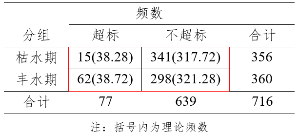
Warning in chisq.test(mt): Chi-squared approximation may be incorrect


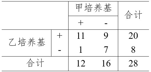
    Pearson's Chi-squared test with Yates' continuity correction

data:  mt
X-squared = 3.444, df = 1, p-value = 0.06348

检验结果发现接受H₀，但p接近检验水准\alpha，改用Fisher精确检验：

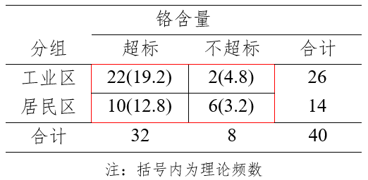
fisher.test(mt)


    Fisher's Exact Test for Count Data

data:  mt
p-value = 0.04204
alternative hypothesis: true odds ratio is not equal to 1
95 percent confidence interval:
  0.9160508 73.9370368
sample estimates:
odds ratio 
  6.266107

Fisher精确检验结果结果拒绝H₀。

(2)列联表资料的独立性检验
列联表资料的独立性检验是检验两个变量是否独立，亦即是否存在相关性，R中采用\chi^2检验方法，即chisq.test()函数。由于该函数亦可用于方差齐性检验，这让人容易混淆对独立性检验与方差齐性检验的理解，二者实际上存在本质区别：齐性检验是对不同总体分别抽样，而独立性检验是对同一总体进行抽样再分类；齐性检验基于各总体在某个变量不同分类上是否具有相同概率的假设，而独立性检验是基于事件独立的假设；齐性检验中的变量关系不对等，可分为自变量和因变量，而独立性检验中的变量关系平等。

例 4.33 某地水源受氟污染，为掌握氟污染对人体健康的危害，有关机构在2010年对该地区1176人进行了调查，发现802人患有釉斑症，各级发病程度与饮用水氟含量的频数资料如下表所示。试问饮用水氟含量与釉斑症的发病程度的有无相关性(独立性检验)？

解：H₀为饮用水氟含量与釉斑病发病程度无关，H₁为饮用水氟含量与釉斑病发病程度有关；

mt = matrix(c(39, 87, 87, 33, 58, 75, 157, 66, 14, 28, 69, 89),
            nrow = 4, dimnames = list("氟含量" = paste0("C", 1:4),
                                "发病程度"=c("初显症","1度","2~3度")))
chisq.test(mt)


    Pearson's Chi-squared test

data:  mt
X-squared = 88.424, df = 6, p-value < 2.2e-16

检验结果拒绝H₀，表明饮用水氟含量与釉斑病发病程度有关。

(3)配对列联表资料的McNemar检验
对于配对的二维列联表资料，如每一对实验对象给予不同的处理，或同一实验对象先后给予不同的处理，McNemar检验通过频数变化来检验一致性，R中函数为mcnemar.test()。

例 4.34 将28份微生物样品按相同条件分别接种于甲乙两种培养基，“+”表示能够生长，“-”表示不能生长，最终接种培养结果整理汇总于下表中。试问两种培养基效果是否一致？

解：H₀为两种培养基效果一致，H₁为两种培养基效果不一致；

mt = matrix(c(11, 1, 9, 7), nrow=2,
            dimnames = list("乙培养基" = c("阳性", "阴性"),
                            "甲培养基" = c("阳性", "阴性")))
mcnemar.test(mt, correct = TRUE)


    McNemar's Chi-squared test with continuity correction

data:  mt
McNemar's chi-squared = 4.9, df = 1, p-value = 0.02686

结果拒绝H₀，表明两种培养基效果不一致，乙培养基的效果优于甲培养基。

4.2.3.7 分布函数的拟合优度检验

拟合优度(goodness-of-fit)检验用于检验样本所在总体的分布与某一理论分布是否一致。令某总体的分布函数为F(x)且未知，X为来自该总体的一个样本，x_i(i=1\sim n)为观测值。则该类问题的假设为：H₀为F(x)=F_0(x,\theta)，H₁为F(x)≠F_0(x,\theta)，其中\theta是分布的未知参数，在检验之前，需要对其进行估计。

(1)Shapiro-Wilk正态性检验
该方法也称W检验，用于检验样本是否来自于正态总体，对异常值敏感，适用于小样本。R中执行该检验的函数为shapiro.test()。

例 4.35 Shapiro-Wilk正态性检验示例。

x = rnorm(100, mean = 6, sd = 2)    # 构造正态分布样本
shapiro.test(x)


    Shapiro-Wilk normality test

data:  x
W = 0.99086, p-value = 0.7339

y = runif(100, min = 4, max = 8)    # 构造均匀分布样本
shapiro.test(y)


    Shapiro-Wilk normality test

data:  y
W = 0.97107, p-value = 0.0267

以上代码演示了shapiro.test()函数对不同分布样本的检验，使用简单，检验结果正确。

(2)Kolmogorov-Smirnov检验
该方法简称K-S检验，用于检验样本是否来自某一理论分布，适用于连续型随机变量分布的检验问题。该方法相对稳健，对异常值具有较好的抗干扰能力。R中执行该检验的函数为ks.test()。

例 4.36 Kolmogorov-Smirnov检验示例。

x = rnorm(100, mean = 6, sd = 2)    # 构造正态分布样本
y = runif(80, min = 2, max = 8)    # 构造均匀分布样本
ks.test(x, "pnorm", 6, 2)


    Asymptotic one-sample Kolmogorov-Smirnov test

data:  x
D = 0.057828, p-value = 0.8917
alternative hypothesis: two-sided

检验结果接受H₀，即x来自均值为6、方差为2的正态总体。

ks.test(x, "pnorm", 5, 2)


    Asymptotic one-sample Kolmogorov-Smirnov test

data:  x
D = 0.23281, p-value = 3.92e-05
alternative hypothesis: two-sided

检验结果拒绝H₀，即x不是来自均值为5、方差为2的正态总体。

ks.test(x, y)


    Exact two-sample Kolmogorov-Smirnov test

data:  x and y
D = 0.2125, p-value = 0.03114
alternative hypothesis: two-sided

检验结果表明x和y不是来自同一连续型随机变量分布。

(3)总体分布的Pearson\chi^2检验
Pearson\chi^2检验是最常用的适用于所有理论分布的拟合优度检验方法。可用chisq.test()函数执行该检验，使用时需指定与样本(参数x不能包含负数)等长度的概率向量(参数p，总和必须为1)。

例 4.37 总体分布的Pearson χ2检验示例。

x = runif(10, min = 2, max = 8)    # 构造均匀分布样本
p0 = rep(1 / length(x), length(x))
chisq.test(x, p = p0)


    Chi-squared test for given probabilities

data:  x
X-squared = 6.2747, df = 9, p-value = 0.7121

检验结果表明样本x来自均匀分布总体。

4.2.3.8 其他检验方法

(1)游程检验
游程检验亦称“连贯检验”，是一种非参数检验方法，用于单个样本的随机性或两个总体的分布是否相同。R包tseries中的runs.test()函数可用于二分类或二进制序列的随机性检验。

(2)白噪声检验
白噪声检验也称纯随机性检验，用于检验序列数据是否为纯随机序列，常用于时间序列分析、模型预测残差分析等。R中Box.test()函数用于执行白噪声检验。

(3)Wilcoxon秩和检验和Wilcoxon符号秩检验
秩(rank)是样本中变量观测值从小到达排序后的次序号。Wilcoxon秩和检验和Wilcoxon符号秩检验都是利用样本数据的秩信息进行检验，属于非参数检验方法，用于不能满足t检验的场景，如总体分布不是正态分布，或总体分布类型未知。R中wilcox.test()函数执行这两种检验，其中参数paired默认为FALSE，执行Wilcoxon秩和检验；当paired设置为TRUE，则执行配对资料的Wilcoxon符号秩检验。pairwise.wilcox.test()函数执行两两比较的秩和检验和符号秩检验。

(4)Kruskal-Wallis秩和检验(K-W检验)
K-W检验是用于三个及三个以上独立样本是否来自相同分布的非参数检验方法，前提要求总体是连续型分布，除位置参数不同外，分布相似。R中kruskal.test()函数执行该检验。

(5)Friedman检验
Friedman检验也是检验三个及三个以上独立样本是否来自相同分布的非参数检验方法，但要求样本为配对资料。R中friedman.test()函数执行该检验。

(6)Bartlett、Levene及Fligner-Killeen方差齐性检验
三者都是多样本方差齐性检验的方法，Bartlett方法为参数检验方法，用于正态分布数据，R中函数为bartlett.test()；Levene方法是非参数检验方法，可用于非正态分布数据，R中函数为car包中的leveneTest()函数；Fligner-Killeen方法也是非参数检验方法，R中函数为fligner.test()。

R及很多R包提供了针对各种场景下的假设检验函数，具体使用可根据需要查询相关函数或R包的使用方法。

4.2.3.9 方差分析

在环境科学与工程研究工作中，经常需要同时对三个及三个以上的样本均值进行比较，如比较不同工艺去除污染物的效果，比较不同污染物的毒性等，比较不同季节大气中某种污染物的含量等。这里研究的工艺、污染物种类、污染物、季节即为因素(也称为控制变量，)，因素所处的状态称为水平，而研究者感兴趣的污染物去除效果、毒性、含量称为观测变量或研究变量。应用t检验分析多样本均值差异的显著性需要执行很多次，且容易增大分析误差，而应用方差分析(F检验法)可简化分析步骤。除此以外，方差分析还有很多用途，如分析多个因素之间的交互作用、回归模型的显著性检验等。

方差分析的前提要求是样本必须满足独立性、正态性和方差齐性。独立性是指各样本来自相互独立的随机总体，正态性是指各样本均来自正态总体，方差齐性是指各样本对应总体的方差相同。方差分析的基本思想是把全部观测值的总变异，按因素分组进行分析，计算每个因素对总变异的贡献，从而判定因素的重要性。例如，在单因素的完全随机设计的实验资料中，总变异可分为组内变异和组间变异；在配伍组设计的资料中，总变异可分为处理组间变异、配伍组间变异及误差三部分；在2×2析因设计资料中，总变异可分为两个因素的两个组间变异、两因素交互作用及误差四部分。

R中执行方差分析的函数为aov()，该函数的形式如下：

aov(formula, data = NULL, projections = FALSE, qr = TRUE,
    contrasts = NULL, ...)

formula是一个用公式指定的模型，如”y ~ x”，“y ~ a + b + c”，“y ~ a + b + a:b”等。其中常用的符号及其意义如表 4.3 所示。data是包含所有变量的数据框。projections为逻辑值，指定是否返回投影。qr为逻辑值，指定是否返回QR分解结果。contrasts是用于公式中某些因素的对比列表。…是传递给线性模型lm()函数的其他参数。

表 4.3: R中formula中常用的符号及其意义

符号	含义
~	左边为因变量，右边为自变量。例如通过a、b和c预测y，代码为y ~ a + b + c
+	分隔自变量
:	表示自变量的交互项。例如通过a、b及其交互项预测y，代码为y ~ a + b + a:b
*	表示所有可能交互项的简洁方式。例如y ~ a * b * c等价于y ~ a + b + c + a:b + b:c + c:a
^	表示交互项达到某个次数。例如y ~ (a + b + c)^2等价于y ~ (a + b + c) * (a + b + c)
.	点号，表示包含除因变量外的所有变量。例如数据包含变量y、a、b和c，代码y ~ . 等价于y ~ a + b + c
-	表示从等式中移除某个变量。例如y ~ (a + b + c)^2 – a:b等价于y ~ a + b + c + b:c + c:a
%in%	表示其左侧项嵌套如右侧项中。如y ~ a + b %in% a等价于y ~ a + a:b
-1或+0	删除截距项。例如y ~ a - 1或y ~ a + 0，强制直线方程通过原点
函数I()	避免公式中算术运算符和符号运算符产生混淆。例如y ~ a + (b + c)^2等价于y ~ a + b + c + b:c；相反, y ~ a + I((b + c)^2)等价于y ~ a + h，h是b与c之和的平方
函数引用	可以在表达式中用的数学函数。例如log(y) ~ a + b + c表示通过a、b和c来预测log(y)

(1)单因素方差分析(one-way ANOVA)
单因素方差分析就是研究一个因素的多个水平对观测变量是否产生显著性影响。

例 4.38 某湖不同季节湖水中氯化物含量(mg/L)监测结果如下所示。试问不同季节湖水的氯化物含量的差异有无显著意义？
春：22.6, 22.8, 21.0, 16.9, 24.0, 21.9, 21.5, 21.2
夏：19.1, 22.8, 24.5, 18.0, 15.2, 18.4, 20.1, 21.5
秋：18.9, 13.6, 17.2, 15.1, 16.6, 14.2, 16.7, 19.6
冬：19.0, 16.9, 17.6, 14.8, 13.1, 16.9, 16.2, 14.8

解：全部32个观测值之间的总变异包括了季节的影响以及随机误差；4个季节均值之间的差异是组间变异，反映了季节对湖水氯化物含量的可能影响，但也有随机误差的贡献；每个季节内8个观测值之间的差异是组内变异，与季节无关，反映的是随机误差的影响。

library(tidyverse)
# 宽表
df = data.frame(
  春 = c(22.6, 22.8, 21.0, 16.9, 24.0, 21.9, 21.5, 21.2),
  夏 = c(19.1, 22.8, 24.5, 18.0, 15.2, 18.4, 20.1, 21.5),
  秋 = c(18.9, 13.6, 17.2, 15.1, 16.6, 14.2, 16.7, 19.6),
  冬 = c(19.0, 16.9, 17.6, 14.8, 13.1, 16.9, 16.2, 14.8)
)
# 转换为长表
df = df %>% 
  pivot_longer(cols = everything(),
               names_to = "season",
               values_to = "conc")

ans = aov(conc ~ season, data = df)
summary(ans)

            Df Sum Sq Mean Sq F value   Pr(>F)    
season       3  164.3   54.77    10.4 9.06e-05 ***
Residuals   28  147.4    5.26                     
---
Signif. codes:  0 '***' 0.001 '**' 0.01 '*' 0.05 '.' 0.1 ' ' 1

由结果可知，季节因素对氯化物浓度具有显著影响。
当不满足方差齐性条件时(可用bartlett.test()检验)，使用oneway.test()函数执行方差分析：

oneway.test(conc ~ season, data = df)


    One-way analysis of means (not assuming equal variances)

data:  conc and season
F = 11.423, num df = 3.00, denom df = 15.41, p-value = 0.0003383

结果仍然表明季节对氯化物浓度具有显著影响。
当不满足正态性(可用shapiro.test()检验)和方差齐性(可用car::leveneTest()检验)时，使用kruskal.test()函数：

kruskal.test(conc ~ season, data = df)


    Kruskal-Wallis rank sum test

data:  conc by season
Kruskal-Wallis chi-squared = 16.399, df = 3, p-value = 0.0009392

结果也表明季节对氯化物浓度具有显著影响。

(2)双因素方差分析(two-way ANOVA)
双因素方差分析用于研究两个因素对观测变量有无显著性影响，包括两种类型：不考虑两个因素间的交互作用和考虑两个因素间的交互作用。交互作用是指两个因素存在联合作用，表现为相互促进或相互制约。如果两个因素对观测变量的影响是独立的，不需要考虑交互作用；如果两个因素对观测变量的影响不是独立的，则需要考虑交互作用。开展考虑因素交互作用的方差分析，要求两个因素的各个水平组合下有重复实验观测值。

例 4.39 某市2016-2017年不同地点不同季节的大气中飘尘浓度(mg/m3)日均值如下表所示：

地点	春	夏	秋	冬
A	0.614	0.475	0.667	1.150
B	0.620	0.420	0.880	1.200
C	0.379	0.200	0.540	0.940

试推断地点和季节两个因素对飘尘浓度有无显著影响。

解：

library(tidyverse)
df = data.frame(
  地点 = LETTERS[1:3],
  春   = c(0.614, 0.620, 0.379),
  夏   = c(0.475, 0.420, 0.200),
  秋   = c(0.667, 0.880, 0.540),
  冬   = c(1.150, 1.200, 0.940)
)
df = df %>% 
  pivot_longer(cols = 2:5, names_to = "季节", values_to = "飘尘浓度")
  
ans = aov(飘尘浓度 ~ 季节 + 地点, data = df)
summary(ans)

            Df Sum Sq Mean Sq F value   Pr(>F)    
季节         3 0.8796 0.29318   88.76 2.32e-05 ***
地点         2 0.1574 0.07871   23.83   0.0014 ** 
Residuals    6 0.0198 0.00330                     
---
Signif. codes:  0 '***' 0.001 '**' 0.01 '*' 0.05 '.' 0.1 ' ' 1

结果表明季节和地点两个因素都对飘尘浓度具有极显著影响，其中季节的影响大于地点的影响。

例 4.40 2015-2016年不同城市不同季节PM_2.5浓度(μg/m^3)月均值如下表所示。试推断城市和季节两个因素及二者交互项对PM_2.5浓度有无显著影响(假定数据符合正态性、独立性和方差齐性要求)。

解：将数据整理成csv格式数据文件(本例中文件名为PM2.5-for-annova.csv，编码为UTF-8)，列名分别为pm25、city、month和season。

library(tidyverse)
filename = "./data/PM2.5-for-anova.csv"
df = read_csv(filename, col_names = TRUE, col_types = "nfff", 
              locale = locale(encoding = "UTF-8"))
ans = aov(pm25 ~ city * season, data = df)
summary(ans)

            Df Sum Sq Mean Sq F value   Pr(>F)    
city         5  22497    4499  13.436 3.34e-08 ***
season       3  10894    3631  10.845 1.48e-05 ***
city:season 15   3293     220   0.656    0.813    
Residuals   48  16073     335                     
---
Signif. codes:  0 '***' 0.001 '**' 0.01 '*' 0.05 '.' 0.1 ' ' 1

检验结果表明城市和季节两个因素对PM_2.5浓度具有显著影响，但二者没有交互作用。

当数据不满足正态性和方差齐性条件时，可利用R包rcompanion提供的scheirerRayHare()函数执行Scheirer-Ray-Hare非参数检验：

library(rcompanion)
scheirerRayHare(pm25 ~ city * season, data = df)


DV:  pm25 
Observations:  72 
D:  0.9992765 
MS total:  438

            Df  Sum Sq      H p.value
city         5 17035.6 38.922 0.00000
season       3  5232.4 11.955 0.00754
city:season 15  2859.1  6.532 0.96935
Residuals   48  5948.3

以上数据集中季节变量中的3个月份可视为三次重复。如果是非重复区组设计实验得到的数据，可用friedman.test()进行方差分析。

# A tibble: 24 × 3
# Groups:   season [4]
   season city   pm25
   <fct>  <fct> <dbl>
 1 春     北京   70.7
 2 春     重庆   45.7
 3 春     济南   77.3
 4 春     合肥   61  
 5 春     兰州   47  
 6 春     广州   32.7
 7 夏     北京   55.3
 8 夏     重庆   41.7
 9 夏     济南   68.3
10 夏     合肥   41.3
# ℹ 14 more rows


    Friedman rank sum test

data:  df1$pm25, df1$season and df1$city
Friedman chi-squared = 15, df = 3, p-value = 0.001817

(3)多重比较
当方差分析结果显示差异有显著性，并不代表所有的因素水平间都有显著性差异，此时需要通过多重比较(两两比较)才能明确具体水平间的差异显著性。多重比较的方法有很多，其中R预置了Tukey方法(TukeyHSD()函数)。R包agricolae提供了更多多重比较的方法，除了Tukey方法HSD.test()外，还有LSD方法LSD.test()(最小差数显著法)、Bonferroni方法LSD.test()(设置参数p.adj = “bonferroni”)、SNK方法SNK.test()(也称q检验)、Duncan方法duncan.test()(新复极差法)、Scheffé方法scheffe.test()、Dunnet方法multcomp::glht()等。Tukey方法一般用于较多组(≥6)且容量相同样本的多重比较，较LSD方法保守，不易发现差异显著性。Bonferroni方法般用于5组以下容量相同样本的多重比较。Dunnet方法用于多个实验组与一个对照组的比较。Scheffé方法适用于各种情况下的多重比较，特别是样本容量不同的情况。

例 4.41 对例 4.38 中方差分析的结果做多重比较。

library(agricolae)
library(tidyverse)
# 宽表
df = data.frame(
  春 = c(22.6, 22.8, 21.0, 16.9, 24.0, 21.9, 21.5, 21.2),
  夏 = c(19.1, 22.8, 24.5, 18.0, 15.2, 18.4, 20.1, 21.5),
  秋 = c(18.9, 13.6, 17.2, 15.1, 16.6, 14.2, 16.7, 19.6),
  冬 = c(19.0, 16.9, 17.6, 14.8, 13.1, 16.9, 16.2, 14.8)
)
# 转换为长表
df = df %>% 
  pivot_longer(cols = everything(),
               names_to = "season",
               values_to = "conc")
# 方差分析
model = aov(conc ~ season, data = df)
# R内置的Tukey方法多重比较
out1 = TukeyHSD(model); 
out1

  Tukey multiple comparisons of means
    95% family-wise confidence level

Fit: aov(formula = conc ~ season, data = df)

$season
         diff        lwr      upr     p adj
冬-春 -5.3250 -8.4573904 -2.19261 0.0004083
秋-春 -5.0000 -8.1323904 -1.86761 0.0008718
夏-春 -1.5375 -4.6698904  1.59489 0.5460365
秋-冬  0.3250 -2.8073904  3.45739 0.9918917
夏-冬  3.7875  0.6551096  6.91989 0.0132270
夏-秋  3.4625  0.3301096  6.59489 0.0260275

# agricolae包中Tukey方法多重比较
out2 = HSD.test(model, "season")
out2$groups

      conc groups
春 21.4875      a
夏 19.9500      a
秋 16.4875      b
冬 16.1625      b

# agricolae包中LSD方法多重比较
out3 = LSD.test(model, "season", p.adj = "bonferroni")
out3$groups

      conc groups
春 21.4875      a
夏 19.9500      a
秋 16.4875      b
冬 16.1625      b

TukeyHSD.test()函数的检验结果与agricolae中的HSD.test()函数的结果相同，但结果展示形式不同，前者给出各次比较的均值差的区间估计和p值，后者以字母形式标注组间差异显著性，字母相同表示无显著性差异，字母不同表示有显著性差异。本例中，Bonferroni方法与Tukey方法检验结果一致。
此外，R内置的pairwise.t.test()函数基于t检验方法执行多重比较，并给出p值。

attach(df)
pairwise.t.test(conc, season, p.adjust.method = "bonferroni")


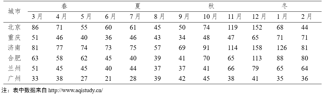
    Pairwise comparisons using t tests with pooled SD 

data:  conc and season 

   春      冬      秋     
冬 0.00044 -       -      
秋 0.00096 1.00000 -      
夏 1.00000 0.01579 0.03223

P value adjustment method: bonferroni

detach(df)

如果需要对因素间交互作用进行可视化，可使用R中interaction.plot()函数，具体使用方法参考该函数的帮助信息。

练习 4.3
四个实验室测定浓度为0.100mg/L的铬标准溶液的结果分别为：A实验室0.099、0.098、0.101、0.099、0.100，B实验室0.099、0.097、0.101、0.098、0.099，C实验室为0.097、0.094、0.098、0.098、0.099，D实验室0.101、0.104、0.101、0.101、0.102。试分析在检验水准为0.01时，四个实验室测定结果是否存在显著性差异？如有显著性差异，进一步开展多重比较。

4.3 相关分析与回归分析

现实世界中，各种因素(变量)交织在一起，相互依赖和制约，数学研究其中的确定性关系——函数关系，而统计学则研究其中的不确定性关系——相关关系。在相关关系分析的基础上，可进一步开展回归分析，建立因变量与其相关的自变量之间的回归模型。

4.3.1 相关分析

4.3.1.1 双变量简单相关系数的计算与检验

相关系数定量地表征两个变量间的线性相关程度及相关方向，其值范围在-1至+1之间，正数为正相关，负数为负相关；绝对值越接近于1表示相关性越高，反之则相关性越低，接近于0为零相关或无相关。

研究两个变量之间的相关关系，可以应用Pearson积矩相关系数(r)、Spearman秩相关系数(\rho)以及Kendall秩相关系数(\tau)。Pearson积矩相关系数基于矩计算，要求两个变量是服从正态分布的连续型变量。Kendall秩相关系数利用原始数据的秩计算，适用于两个定序变量以及不服从正态分布的等间隔数据，是一种非参数统计分析方法。Spearman秩相关系数也利用原始数据的秩计算，适用于连续型和离散型变量，对变量分布类型不作要求，也是一种非参数统计分析方法，可用于使用Pearson积矩相关系数和Kendall秩相关系数的场合，但统计功效低于Pearson积矩相关系数。

R中cor()函数能够计算上述三种相关系数，其中参数method用于设置计算具体相关系数的类型；对于存在缺失值的样本，需要对use参数进行相关设置。对于数据框形式的多变量数据集，cor()函数会给出相关系数矩阵，相关系数矩阵的可视化参见小节 3.4.6.2 相关内容。R中cor.test()函数用于对相关系数进行检验(H₀：相关系数为0)。

在某交通点连续三天监测汽车流量和大气NO₂浓度，每天采样三次，汽车流量(辆/h)监测数据为1500, 960, 1200, 1784, 1176, 1476, 1820, 1060, 1436；NO2浓度(mg/m^3)监测数据为0.1200, 0.0390, 0.1000, 0.2220, 0.1290, 0.1450, 0.1350, 0.0785, 0.0985。试求二者相关系数并进行检验。

x = c(1500, 960, 1200, 1784, 1176, 1476, 1820, 1060, 1436)
y = c(0.1200, 0.0390, 0.1000, 0.2220, 0.1290, 0.1450, 0.1350, 0.0785, 0.0985)
# 计算pearseon相关系数
cor(x, y, method = "pearson")

[1] 0.7988311

# 计算spearman相关系数
cor(x, y, method = "spearman")

[1] 0.7833333

# 计算kendall相关系数
cor(x, y, method = "kendall")

[1] 0.6111111

# 计算pearseon相关系数并进行检验
cor.test(x, y, method = "pearson")


    Pearson's product-moment correlation

data:  x and y
t = 3.5134, df = 7, p-value = 0.009814
alternative hypothesis: true correlation is not equal to 0
95 percent confidence interval:
 0.2869339 0.9558528
sample estimates:
      cor 
0.7988311

检验结果表明pearson相关系数不等于0。

4.3.1.2 多变量偏相关系数的计算与检验

偏相关分析是在三个及以上多变量的相关分析中，在消除其他变量影响的前提下考察两个变量之间的相关关系，因此也称为净相关分析。在三个变量的偏相关分析中，任意两个变量的偏相关系数是消除余下一个变量的影响得到的，称为一阶偏相关系数；在四个变量的偏相关分析中，任意两个变量的偏相关系数称为二阶偏相关系数。以此类推，还有更高阶的偏相关系数，但超过4个变量的情况下，较少采用偏相关分析。

R包ppcor提供了偏相关系数的计算和检验函数：pcor()和pcor.test()。下面对R内置数据集airquality的前四个变量(Ozone、Solar.R、Wind、Temp)进行相关分析和偏相关分析。

例 4.42 对airquality数据集进行相关和偏相关分析。

library(ppcor)
library(dplyr)
df = airquality %>% 
  dplyr::select(Ozone:Temp) %>% 
  na.omit()
# 计算简单相关系数
cor(df, method = "spearman")

             Ozone     Solar.R        Wind       Temp
Ozone    1.0000000  0.34818647 -0.60513642  0.7729319
Solar.R  0.3481865  1.00000000 -0.06169636  0.2095369
Wind    -0.6051364 -0.06169636  1.00000000 -0.4993228
Temp     0.7729319  0.20953692 -0.49932278  1.0000000

# 计算偏相关系数
pcor(df, method = "spearman")

$estimate
             Ozone     Solar.R        Wind        Temp
Ozone    1.0000000  0.34980011 -0.43451018  0.66817934
Solar.R  0.3498001  1.00000000  0.19474883 -0.08967312
Wind    -0.4345102  0.19474883  1.00000000 -0.04363683
Temp     0.6681793 -0.08967312 -0.04363683  1.00000000

$p.value
               Ozone      Solar.R         Wind         Temp
Ozone   0.000000e+00 0.0001926827 2.349034e-06 2.064670e-15
Solar.R 1.926827e-04 0.0000000000 4.243081e-02 3.537753e-01
Wind    2.349034e-06 0.0424308090 0.000000e+00 6.523181e-01
Temp    2.064670e-15 0.3537753412 6.523181e-01 0.000000e+00

$statistic
            Ozone    Solar.R       Wind       Temp
Ozone    0.000000  3.8623681 -4.9903112  9.2899174
Solar.R  3.862368  0.0000000  2.0538218 -0.9313381
Wind    -4.990311  2.0538218  0.0000000 -0.4518132
Temp     9.289917 -0.9313381 -0.4518132  0.0000000

$n
[1] 111

$gp
[1] 2

$method
[1] "spearman"

从计算结果可以发现，Ozone与Solar.R、Wind和Temp三个变量的偏相关系数都具有显著性，其中与Solar.R的偏相关系数比简单相关系数略有增大，而与Wind和Temp两个变量的偏相关强度都有所减弱。因此，多变量的两两变量相关分析应采用偏相关分析，以消除其他变量的影响，从而真实呈现两两变量之间的相关性。

4.3.1.3 多变量复相关系数的计算与检验

在三个及以上多变量的相关分析中，复相关分析是要考察其中一个变量y(因变量)受其他一组变量x_i(自变量)的综合影响。采用复相关系数(亦称多重相关系数)来量化表征一个变量与一组变量之间的相关程度，其取值范围为[0, 1]。复相关分析常用于多元线性回归分析。

计算复相关系数需要先建立y与x_i的多元线性回归方程，再基于多元线性回归方程代入x_i的观测值，计算出y的预测值\hat{y}，然后计算y与\hat{y}的简单相关系数即为y与x_i的复相关系数。例 4.43 演示了R中三种计算复相关系数的方法。

例 4.43 计算airquality数据集中Ozone变量与Solar.R、Wind和Temp三个变量的复相关系数。

library(dplyr)
df = airquality %>% 
  dplyr::select(1:4) %>% 
  na.omit()
fm = lm(Ozone ~ ., data = df)
y = df$Ozone
yp = fm$fitted.values
R1 = cor(y, yp)
R1

[1] 0.7783923

R2 = cov(y, yp)/sqrt(var(y) * var(yp))
R2

[1] 0.7783923

R3 = sqrt(summary(fm)$r.sq)
R3

[1] 0.7783923

以上三种方法的计算结果完全一致，其中第二种方法借助协方差计算函数cov()，第三种方法是取回归模型的决定系数(R^2)的平方根。

rstatix和easystats是与tidyverse设计理念一致的tidy风格的统计分析工具包，整合了R及相关工具包的统计分析与推断的功能，具体功能和使用可阅读相关帮助信息。

练习 4.4
基于R内置数据集mtcars，选择mpg、disp、hp、drat、wt和qsec等6个变量，
(1)计算两两相关系数矩阵并绘制相关系数矩阵图；
(2)计算mpg、wt和qsec之间偏相关系数；
(3)计算mpg与其他5个变量的复相关系数。

4.3.2 回归分析

回归分析是一种定量描述变量间相互依赖关系的统计分析方法，常用于截面数据。一个自变量(也称预测变量)与一个因变量(也称响应变量)之间的回归分析称为一元回归分析(也称简单回归分析)，多个自变量与一个因变量之间的回归分析称为多元回归分析(也称多重回归分析)。根据自变量与因变量之间的关系类型，可分为线性回归分析和非线性回归分析。

相关分析只是定量描述了变量间相关关系的性质和程度，回归关系则是定量描述变量间相关依赖的函数形式。相关分析是回归分析的基础和前提，回归分析是相关分析的深入和继续，能够量化解释因变量对自变量的依赖性质和程度，并可在一定范围内进行预测。

4.3.2.1 线性回归

线性回归是在因变量和自变量之间建立如下的线性回归模型：

Y = X \cdot \beta + \epsilon \tag{4.29}

其中Y为因变量，X为自变量(包含一个或多个自变量)，\beta为回归系数(也称权重)\epsilon为随机误差，且假定\epsilon \sim N(0,\sigma)。每个自变量对应回归系数的符号(正或负)表明该自变量和因变量之间相关关系的方向，每个自变量的回归系数的绝对值表示在模型中其他自变量保持不变的情况下，该自变量变化一个单位，因变量的平均值就会发生多大的变化。

R中lm()函数用于求解回归系数，其算法是基于普通最小二乘法(OLS)。该函数和aov()函数一样采用formula参数来指定因变量和自变量。

例 4.44 以airquality数据集中Ozone为因变量、Solar.R为自变量建立一元线性回归模型。

fm = lm(Ozone ~ Solar.R, data = airquality)
summary(fm)


Call:
lm(formula = Ozone ~ Solar.R, data = airquality)

Residuals:
    Min      1Q  Median      3Q     Max 
-48.292 -21.361  -8.864  16.373 119.136 

Coefficients:
            Estimate Std. Error t value Pr(>|t|)    
(Intercept) 18.59873    6.74790   2.756 0.006856 ** 
Solar.R      0.12717    0.03278   3.880 0.000179 ***
---
Signif. codes:  0 '***' 0.001 '**' 0.01 '*' 0.05 '.' 0.1 ' ' 1

Residual standard error: 31.33 on 109 degrees of freedom
  (42 observations deleted due to missingness)
Multiple R-squared:  0.1213,    Adjusted R-squared:  0.1133 
F-statistic: 15.05 on 1 and 109 DF,  p-value: 0.0001793

summary()给出的摘要信息中，Call部分显示了函数调用形式，Residuals部分给出了模型残差最小和最大值以及四分位数，Coefficients部分给出了回归系数的估计值、标准差、t检验统计量和显著性检验的p值，其中Intercept为截距(亦称回归常数，即\beta_0)，接下来是各个自变量的回归系数。最后一段信息给出了残差标准差和自由度、模型决定系数(\text{R}^2)和校正决定系数(\text{R}_a^2)以及模型显著性检验(F检验)的结果；如有缺失值，还会给出因数据缺失而删除的观测数。

每个自变量回归系数的p值大于检验水准时，即没有显著性意义，表明样本不足以拒绝在总体上该自变量与因变量之间相关性为零的原假设；当p值小于检验水准时，即有显著性意义，则表明样本足以拒绝在总体上该自变量与因变量之间相关性为零的原假设，该自变量可能值得添加到回归模型中。决定系数\text{R}^2是自变量能够解释因变量变异的部分与因变量总变异的比例，即

\text{R}^2 = \frac {\sum{(\hat {y}_i - \bar{y})^2}} {\sum{(y_i - \bar{y})^2}} = 1 - \frac {\sum{(\hat {y}_i - y_i)^2}} {\sum{(y_i - \bar{y})^2}} \tag{4.30}

\text{R}^2常用于回归方程拟合优度的评价，但其只是相关性而非准确性的度量指标。随着回归方程中自变量个数的增加，\text{R}^2会出现过高的估计，为此提出考虑自变量个数的\text{R}_a^2，以避免对回归方程拟合优度的乐观估计(\text{R}_a^2总是小于\text{R}^2)。总是假定样本内观测数为n，每个观测的变量数为k，则

\text{R}_a^2 = 1 - \frac {\sum{(\hat {y}_i - y_i)^2}/(n-k-1)} {\sum{(y_i - \bar{y})^2}/(n-1)} = 1 - (1 - \text{R}^2) \frac {n-1} {n-k-1} \tag{4.31}

另一个\text{R}_a^2的计算公式是将上式中(n-p-1)改为(n-p)，这在一个自变量的情况下，\text{R}_a^2 = \text{R}^2。

从例 4.44 中summary()函数的摘要结果来看，回归模型和两个回归系数都具有显著意义，但从\text{R}^2来看，模型的拟合优度很低。下面，将Temp和Wind变量引入回归模型，观察回归系数和决定系数的变化。

例 4.45 以airquality数据中的Ozone为因变量，以 Solar.R、Temp及Wind为自变量，建立多元回归模型。

fm1 = lm(Ozone ~ Solar.R + Temp + Wind, data = airquality)
summary(fm1)


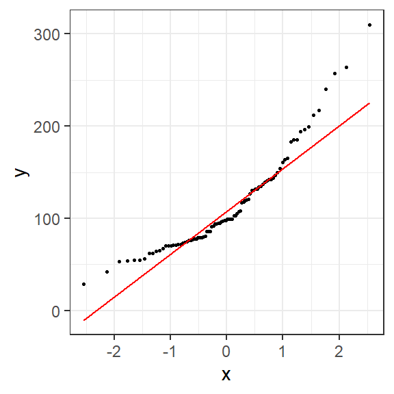
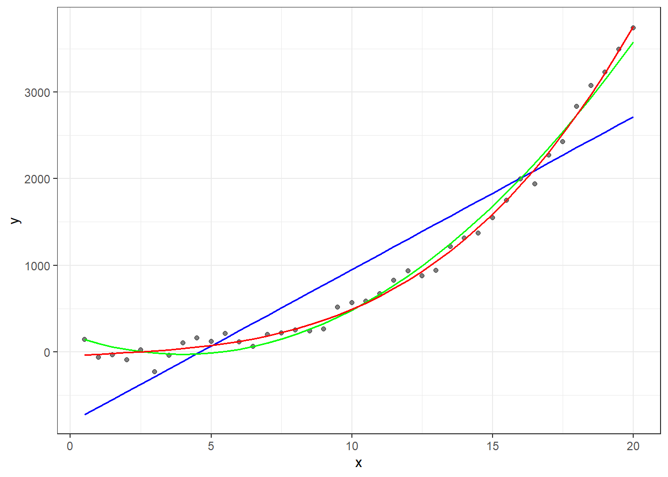
Call:
lm(formula = Ozone ~ Solar.R + Temp + Wind, data = airquality)

Residuals:
    Min      1Q  Median      3Q     Max 
-40.485 -14.219  -3.551  10.097  95.619 

Coefficients:
             Estimate Std. Error t value Pr(>|t|)    
(Intercept) -64.34208   23.05472  -2.791  0.00623 ** 
Solar.R       0.05982    0.02319   2.580  0.01124 *  
Temp          1.65209    0.25353   6.516 2.42e-09 ***
Wind         -3.33359    0.65441  -5.094 1.52e-06 ***
---
Signif. codes:  0 '***' 0.001 '**' 0.01 '*' 0.05 '.' 0.1 ' ' 1

Residual standard error: 21.18 on 107 degrees of freedom
  (42 observations deleted due to missingness)
Multiple R-squared:  0.6059,    Adjusted R-squared:  0.5948 
F-statistic: 54.83 on 3 and 107 DF,  p-value: < 2.2e-16

显然，引入两个新的自变量后，新模型的回归系数和决定系数都发生了变化，其中截距变为负值且绝对值增大，而Solar.R的回归系数明显减小。此外，\text{R}^2明显增大，残差减小，说明回归模型的拟合优度得到了改善。从例 4.45 的结果可以发现，新引入的自变量Temp和Wind与因变量Ozone的相关性更高，对其影响大于Solar.R。

回归模型建立后，除了利用summary()函数提取模型摘要信息外，还可以通过以下函数提取其他信息以进一步分析:

coefficients(): 提取回归模型的回归系数
residuals(): 提取回归模型的残差
confint(): 计算回归系数的置信区间(默认 95%)
fitted(): 计算回归模型对建模数据集的拟合值
anova(): 计算回归模型的方差分析表
AIC(): 计算赤池信息统计量
BIC(): 计算贝叶斯信息统计量
plot(): 生成回归模型的诊断图形
predict(): 利用回归模型对新数据集进行预测

例如，利用confint()获取例 4.45 中多元回归模型的回归系数的置信区间：

confint(fm1)

                    2.5 %      97.5 %
(Intercept) -110.04538108 -18.6387768
Solar.R        0.01385613   0.1057851
Temp           1.14949967   2.1546862
Wind          -4.63087706  -2.0363055

回归系数体现了自变量变化对因变量的影响方向和程度，是回归模型解释功能的重要部分。
predict()基于已经建立的回归模型，用新的自变量数据预测对应的因变量的值。对于线性回归模型，该函数提供点预测和区间预测两种功能，执行区间预测只需设置参数interval和level值即可。interval设置为”confidence”时，计算置信区间(窄区间)，设置为”prediciton”时，计算公差区间(宽区间)。level默认值是0.95，即计算置信概率为95%的区间。

set.seed(2023)
new_data = data.frame(
  Solar.R = sample(na.omit(airquality$Solar.R), 5),
  Temp = sample(na.omit(airquality$Temp), 5),
  Wind = sample(na.omit(airquality$Wind), 5)
)
new_data

  Solar.R Temp Wind
1     167   81 10.3
2     190   65 13.8
3     223   92 11.5
4     284   73  9.7
5     273   82  7.4

# 点预测
predict(fm1, newdata = new_data)

        1         2         3         4         5 
45.131495  8.406312 62.654160 40.913915 62.791985

# 窄区间预测
predict(fm1, newdata = new_data, interval = "confidence")

        fit      lwr      upr
1 45.131495 40.56799 49.69500
2  8.406312  1.20245 15.61018
3 62.654160 53.64414 71.66418
4 40.913915 33.89565 47.93218
5 62.791985 56.71742 68.86655

# 宽区间预测
predict(fm1, newdata = new_data, interval = "prediction")

        fit        lwr       upr
1 45.131495   2.895862  87.36713
2  8.406312 -34.195550  51.00818
3 62.654160  19.709970 105.59835
4 40.913915  -1.656956  83.48479
5 62.791985  20.366481 105.21749

需要注意的是，新数据集中变量名必须与建立回归模型的变量名一致。另外，预测使用的新数据，严格意义上，各自变量的值应在建立回归模型使用的自变量值域内，否则预测的准确性将难以保证。

除了对因变量进行预测，线性回归模型还可以反过来对自变量进行控制，即在确保因变量在某个概率下的置信区间时，如何控制自变量的取值范围，亦即反预测。一元线性回归模型的控制相对简单，但多元线性回归的控制就很复杂，有兴趣的读者可研读相关文献资料。

在多元线性回归中，经常需要考虑自变量之间的交互作用，这可以利用符号”:“或”*“来实现，例如考虑例 4.45 中回归模型中Wind和Temp的交互作用对Ozone的影响：

fm2 = lm(Ozone ~ Solar.R + Temp * Wind, data = airquality)
summary(fm2)


Call:
lm(formula = Ozone ~ Solar.R + Temp * Wind, data = airquality)

Residuals:
    Min      1Q  Median      3Q     Max 
-38.888 -11.938  -3.084   8.753  94.235 

Coefficients:
              Estimate Std. Error t value Pr(>|t|)    
(Intercept) -245.08368   46.84632  -5.232 8.53e-07 ***
Solar.R        0.06599    0.02152   3.067 0.002745 ** 
Temp           3.91373    0.57217   6.840 5.26e-10 ***
Wind          14.38471    4.13249   3.481 0.000727 ***
Temp:Wind     -0.22795    0.05259  -4.334 3.34e-05 ***
---
Signif. codes:  0 '***' 0.001 '**' 0.01 '*' 0.05 '.' 0.1 ' ' 1

Residual standard error: 19.61 on 106 degrees of freedom
  (42 observations deleted due to missingness)
Multiple R-squared:  0.6652,    Adjusted R-squared:  0.6526 
F-statistic: 52.66 on 4 and 106 DF,  p-value: < 2.2e-16

结果表明Temp和Wind交互项的回归系数具有显著性，这表明因变量与其中一个自变量的关系依赖于另外一个自变量的水平，例如Ozone与Temp的关系依Wind不同而不同。同时，模型残差进一步减小，\text{R}^2也增大了一些。

4.3.2.2 非线性回归

非线性关系在现实世界中极为普遍，其中一些非线性关系可以通过数学变换(如对数变换)转变为线性关系，称之为本质线性关系；而无法通过数学变换将其转化为线性关系的，则称之为本质非线性关系。对于前一种情况，对变量进行数学变换，然后对变换后的新变量建立线性回归模型。对于后者，则需要采用非线性回归算法进行建模。

尽管本质线性关系的非线性问题可以使用线性回归模型，但往往会降低模型的可解释性。例如一级动力学方程C_t=C_t e^{-kt} 、米氏方程v_0=v_{max} C/(k_m+C)等，按其方程固有形式估计出的参数都有清晰的解释，如一级动力学模型中k是反应速率，米氏方程中的v_{max}是指最大反应速率。

统计分析中，可以利用多项式回归、样条回归、广义加法模型(GAM)等方法来拟合变量间的非线性关系，这里仅介绍基于lm()函数的多项式回归。

例 4.46 基于一个三次多项式方程构造一个包含50个观测的数据集，然后分别建立直线回归、2阶多项式回归和3阶多项式回归模型，并对拟合结果进行可视化。

library(tidyverse)
# 构造数据集
set.seed(2022)
x = seq(0.5, 20, by = 0.5)
df = data.frame(
  x = x,
  y = 20 + 0.5 * (x - 0.5)^3 + rnorm(40, mean = 30, sd = 100)
)
# 绘制散点图
p = ggplot(df,aes(x = x, y = y)) +
  geom_point(size = 1.5, alpha = 0.5) + theme_bw()
# 建立直线回归方程并可视化拟合结果
fm1 = lm(y ~ x, data = df)
# 绘制fm1的拟合曲线
p = p + geom_line(aes(x, fitted(fm1)), size = 0.6, color = "blue")
# 建立2阶多项式回归方程并可视化拟合结果
fm2 = lm(y ~ poly(x, 2), data = df)
# 绘制fm2的拟合曲线
p = p + geom_line(aes(x, fitted(fm2)), size = 0.6, color = "green")
# 建立3阶多项式回归方程并可视化拟合结果
fm3 = lm(y ~ poly(x, 3), data = df)
# 绘制fm3的拟合曲线
p = p + geom_line(aes(x, fitted(fm3)), size = 0.6, color = "red")
p

下面利用anova()函数对三个模型进行显著性检验：

anova(fm1, fm2, fm3)

Analysis of Variance Table

Model 1: y ~ x
Model 2: y ~ poly(x, 2)
Model 3: y ~ poly(x, 3)
  Res.Df     RSS Df Sum of Sq      F    Pr(>F)    
1     38 7512978                                  
2     37  520393  1   6992585 900.96 < 2.2e-16 ***
3     36  279405  1    240988  31.05 2.593e-06 ***
---
Signif. codes:  0 '***' 0.001 '**' 0.01 '*' 0.05 '.' 0.1 ' ' 1

结果表明直线回归模型fm1没有显著性，而2阶和3阶多项式回归模型fm2和fm3都具有显著性。

很多领域针对特定问题已经建立了相应的数学模型，如一级动力学方程、米氏方程等，这类问题需要估计模型参数，此时，可以用R中基于非线性最小二乘法的函数nls()来解决。该函数通过迭代来求解参数，一般需要根据经验预先设定参数初始值：

model = nls(y ~ a * exp(b * x), data = df, start = list(a = ..., b = ...), ...)

参数初始值对迭代计算具有极大影响，其设定需要经验，主观性太强。为此，R提供了部分常用方程的自启动模型(Self-Satrt models)，避免人为设置初始参数。输入?selfStart，即可打开关于自启动模型的帮助页面，查询相关自启动模型参数设置的函数。下面是其中的部分自启动模型函数：
- SSfol(Dose, input, lKe, lKa, lCl)：一级动力学房室模型
- SSbiexp(input, A1, lrc1, A2, lrc2)：双指数模型
- SSgompertz(x, Asym, b2, b3)：Gompertz增长曲线模型
- SSlogis(input, Asym, xmid, scal)：逻辑斯蒂曲线模型
- SSmicmen(input, Vm, K)：米氏方程模型

例如，对米氏方程采用自启动模型：fit = nls(y ~ SSmicmen(x, vm, k), data = df)。

例 4.47 利用nls函数求解一级动力学方程的参数。

# 构造数据集
set.seed(2022)
x = seq(0, 20, length.out = 40)
df = data.frame(
  x = x,
  y = 5.5 * exp(-0.52 * x) + rnorm(40, 0.08, 0.2))
# 用nls求解参数
fm = nls(y ~ a * exp(-b * x), data = df,
         start = c(a = 1, b = 0.1)) 
summary(fm)


Formula: y ~ a * exp(-b * x)

Parameters:
  Estimate Std. Error t value Pr(>|t|)    
a  5.54533    0.15719   35.28   <2e-16 ***
b  0.53944    0.02468   21.86   <2e-16 ***
---
Signif. codes:  0 '***' 0.001 '**' 0.01 '*' 0.05 '.' 0.1 ' ' 1

Residual standard error: 0.1921 on 38 degrees of freedom

Number of iterations to convergence: 7 
Achieved convergence tolerance: 1.491e-06

# 绘制拟合图形
ggplot(df) +
  geom_point(aes(x,y),size = 1, alpha = 0.5) +
  geom_line(aes(x, fitted(fm)),color = "red") +
  theme_bw()

从摘要信息中可见，参数a和b的求解结果非常接近于前面构造数据所使用的参数值；从拟合图形可见拟合程度较好。

4.3.2.3 线性回归模型诊断与改善方法

基于OLS的线性回归模型有以下六个假设：
(1)线性：因变量和自变量之间满足线性关系；
(2)可加性：不同自变量对因变量的影响可直接相加；
(3)独立性：自变量之间互不相关；反之，自变量之间存在多重共线性；
(4)随机性：残差序列完全随机，特别是时间序列数据；反之，残差存在自相关；
(5)正态性：残差满足正态分布；
(6)方差齐性：残差的方差为常数，也称同方差性。

线性回归模型诊断包括模型残差分析(检验随机性、正态性和方差齐性)、自变量多重共线性分析以及其他影响因素的分析。

plot()可以绘制线性回归模型(lm()返回的对象)的4个诊断图形，对残差的随机性(反映自变量与因变量有无线性关系)、正态性、方差齐性以及离群点(模型拟合误差很大的数据点)、强影响点(对模型参数估计影响过大的数据点)和高杠杆值点(自变量空间中的离群点，因变量不参与计算)，但无法检验独立性和多重共线性。

car包提供了更丰富的诊断函数，其中qqPlot()绘制分位数比较图检验正态性，crPlot()绘制残差成分与残差图执行残差分析，durbinWatsonTest()检验残差的随机性，ncvTest()检验残差的方差齐性，spreadLevelPlot()绘制拟合值与残差图来判断残差的方差齐性，outlierTest()检验离群点，influencePlot()绘制残差与帽子值(hat统计量)的气泡图来显示离群点、强影响点和高杠杆值点，vif()计算方差膨胀因子来检验多重共线性。

gvlma包中的gvlma()函数可以对线性模型的假设进行全局验证，同时检验偏度、峰度和异方差性。该函数返回的结果中，Global Stat项的决策结果直接给出该线性模型是否通过了综合检验。

例 4.48 利用gvlma函数对例 4.46 中fm2和fm3模型进行综合检验。

library(gvlma)
gvlma(fm2)


Call:
lm(formula = y ~ poly(x, 2), data = df)

Coefficients:
(Intercept)  poly(x, 2)1  poly(x, 2)2  
      993.5       6445.6       2644.3  


ASSESSMENT OF THE LINEAR MODEL ASSUMPTIONS
USING THE GLOBAL TEST ON 4 DEGREES-OF-FREEDOM:
Level of Significance =  0.05 

Call:
 gvlma(x = fm2) 

                      Value   p-value                   Decision
Global Stat        21.41383 2.621e-04 Assumptions NOT satisfied!
Skewness            0.28416 5.940e-01    Assumptions acceptable.
Kurtosis            1.38066 2.400e-01    Assumptions acceptable.
Link Function      19.72332 8.950e-06 Assumptions NOT satisfied!
Heteroscedasticity  0.02569 8.727e-01    Assumptions acceptable.

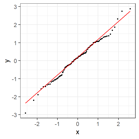
gvlma(fm3)


Call:
lm(formula = y ~ poly(x, 3), data = df)

Coefficients:
(Intercept)  poly(x, 3)1  poly(x, 3)2  poly(x, 3)3  
      993.5       6445.6       2644.3        490.9  


ASSESSMENT OF THE LINEAR MODEL ASSUMPTIONS
USING THE GLOBAL TEST ON 4 DEGREES-OF-FREEDOM:
Level of Significance =  0.05 

Call:
 gvlma(x = fm3) 

                    Value p-value                Decision
Global Stat        5.3380  0.2543 Assumptions acceptable.
Skewness           1.3014  0.2540 Assumptions acceptable.
Kurtosis           0.2838  0.5942 Assumptions acceptable.
Link Function      1.6340  0.2012 Assumptions acceptable.
Heteroscedasticity 2.1188  0.1455 Assumptions acceptable.

检验结果表明，二阶多项式模型fm2不满足假设，而三阶多项式模型fm3符合假设。

对于有很多自变量的多元线性回归模型，需要检验多重共线性。此时可以先借助car包中vif()计算出模型中每个自变量的VIF值，然后对其取平方根(sqrt()函数)，结果大于2的变量被认为存在多重共线性。

改善线性回归模型的方法包括：
(1)删除离群点和强影响点，删除后需要重新建立回归模型；或采用稳健回归(MASS包中的rlm()函数)；
(2)存在多重共线性的，可以采取逐步回归法(step()函数或MASS包中的stepAIC()函数)剔除自变量；或采用岭回归方法(ridge regression)或拉索回归(LASSO regression)，这两种回归分析需要借助glmnet包。另一个值得考虑的方法是利用主成分分析提取主成分，然后以主成分作为自变量建立回归模型，或直接采用pls包中的pcr()函数，该包中的plsr()函数执行偏最小二乘回归建模，特别适用于观测数较少而变量数过多的数据；
(3)如果违背正态性假设，可采用非参数回归模型；或采用Box-Cox变量变换方法(car包中powerTransform()函数)；
(4)如果存在异方差性，可利用car包中的spreadLevelPlot()函数来改善；
(4)如果违背线性假设，可采用car包中的boxTidwell()函数来改善；如果存在显著的非线性关系，应采用非线性回归方法；
(5)如果残差存在自相关性，应考虑采用时间序列分析方法或多层次回归方法。

线性混合模型(nlme包)和广义线性模型(glmnet包)可以用于很多不符合普通线性回归假设的情况，可以进一步学习并掌握。另外，quantreg包提供的分位数回归(rq()函数)是一种非参数回归方法，可以估算因变量的条件概率分布。

练习 4.5 基于R内置数据集mtcars，选择mpg、disp、hp、drat、wt和qsec等6个变量，
(1)以mpg为因变量，其他5个变量为自变量，建立多元线性回归模型；
(2)利用gvlma包中的gvlma()函数对模型进行综合检验；
(3)提出改善模型的方法。

4.4 主成分分析与因子分析

主成分分析(PCA)和因子分析(FA)很相似，都是一种多变量降维分析方法。主成分分析属于数学分析方法，而因子分析属于统计分析方法。主成分分析方法主要用来解决多变量多重共线性问题，计算得到的主成分之间互相独立，计算结果唯一，常用于多元回归分析、机器学习建模等，并衍生出主成分回归(PCR)、偏最小二乘回归(PLSR)等回归分析模型。因子分析方法用来探索或验证公共因子的结构模型，重点在于找到并解释现有变量背后的少数控制因素(即公共因子)，而且这些控制因素具有实际意义但往往又难以观测，其计算结果不唯一。

4.4.1 主成分分析

对于高维数据，每一个样本单位(一个观测)的特征(变量)数非常多，甚至多于样本含量(表现为数据表中列数远多于行数)，例如一个样品的红外光谱数据包含上千个波长的吸光度，基因数据的变量也是成千上万。这些变量间存在错综复杂的相关性，很难深入理解，也不能建立稳健的多元回归模型。主成分分析是一种应用广泛的数据降维算法，基于正交变换将n个原始变量转换为n个正交的新变量，即主成分(PCs)。本质上，每个主成分是n个原始变量的线性组合，且各主成分之间互不相关。主成分对数据总方差的解释比例依次从大到小，一般选择累积方差可解释比例(累积贡献率)≥85%的前k(通常k≤3)个主成分数据代表原始数据用于后续的分析与建模，以免丢弃更多原始数据的信息。降维后的k个主成分只丢弃了原始数据的极少部分信息，但带来的好处是消除了数据中冗余的信息，并显著降低后续建模的计算量和模型的复杂度。

主成分分析不要求数据来自正态总体，但要求变量间存在相关性。主成分分析的步骤：
(1)确认原始变量间存在相关性(可使用Bartlett球形检验或Kaiser-Meyer-Olkin检验，对应于R包psych中的cortest.bartlett()函数和KMO()函数)；
(2)对原始数据进行标准化处理以无量纲化；
(3)计算协方差或相关系数矩阵；
(4)基于协方差或相关系数矩阵求解特征值和特征向量；
(5)将特征值从大到小排列，根据累积贡献率确定前k个特征值；
(6)以特征值对应的特征向量为权重构建主成分(以特征向量为权重将原始变量线性组合为新变量)；
(7)计算每个主成分对应的贡献率；
(8)根据主成分的特征值和特征向量进行解释。

实际上，基于原始数据计算得到的相关矩阵，与原始数据标准化处理后计算得到的协方差矩阵相同。

R中内置的princomp()函数和prcomp()函数都可用于主成分分析，前者基于协方差(参数cor = FALSE，输入数据需要标准化处理)或相关系数矩阵(参数cor = TRUE，输入数据不需要标准化处理)进行特征分解得到特征值与特征向量，而后者提供了标准化处理参数，利用奇异值分解(SVD)从原始数据矩阵直接求解特征值与特征向量，计算速度快，在数据规模很大时具有优势，一般作为首选的方法。此外，很多R包如FactoMineR、psych、MASS等都提供了主成分分析功能的函数。factoextra是一个用于对包括主成分分析在内的多元统计分析的结果进行解释和可视化的包。

例 4.49 利用prcomp()对iris数据集进行主成分分析。

df = iris[ , 1:4]
# 相关性检验
library(psych)
cortest.bartlett(cor(df), n = nrow(df))

$chisq
[1] 706.9592

$p.value
[1] 1.92268e-149

$df
[1] 6

根据p值拒绝变量间相关系数为0的假设，说明可以对数据进行主成分分析。

KMO(cor(df))

Kaiser-Meyer-Olkin factor adequacy
Call: KMO(r = cor(df))
Overall MSA =  0.54
MSA for each item = 
Sepal.Length  Sepal.Width Petal.Length  Petal.Width 
        0.58         0.27         0.53         0.63

KMO检验比Bartlett球形检验严格，相关性越高，总MSA(Measure of Sampling Adequacy，抽样充足性测度)值越接近于1，反之则越接近于0，大于0.5即表明存在相关性。

pca_iris = (prcomp(df,scale. = TRUE, center = TRUE))    # 标准化处理
summary(pca_iris)    # 对结果进行摘要

Importance of components:
                          PC1    PC2     PC3     PC4
Standard deviation     1.7084 0.9560 0.38309 0.14393
Proportion of Variance 0.7296 0.2285 0.03669 0.00518
Cumulative Proportion  0.7296 0.9581 0.99482 1.00000

以上结果表明第一个主成分对总方差的解释比例约73%，第二个主成分约23%，二者累计解释比例接近96%，后两个主成分的解释比例很低。因此可选择前2个主成分进行后续的分析与建模。
可用$sdev单独返回标准差(本质上就是对应特征值的平方根)。方差本质上就是对应的特征值，方差比例就是通过特征值计算得到的。返回载荷矩阵通过$rotation：

pca_iris$rotation

                    PC1         PC2        PC3        PC4
Sepal.Length  0.5210659 -0.37741762  0.7195664  0.2612863
Sepal.Width  -0.2693474 -0.92329566 -0.2443818 -0.1235096
Petal.Length  0.5804131 -0.02449161 -0.1421264 -0.8014492
Petal.Width   0.5648565 -0.06694199 -0.6342727  0.5235971

载荷矩阵非常重要，因为通过载荷矩阵，可以将原始变量线性组合成各个主成分，从而得到主成分作为新变量的得分(新观测值)。下面来看主成分作为新变量的前6个观测：

head(pca_iris$x)

           PC1        PC2         PC3          PC4
[1,] -2.257141 -0.4784238  0.12727962  0.024087508
[2,] -2.074013  0.6718827  0.23382552  0.102662845
[3,] -2.356335  0.3407664 -0.04405390  0.028282305
[4,] -2.291707  0.5953999 -0.09098530 -0.065735340
[5,] -2.381863 -0.6446757 -0.01568565 -0.035802870
[6,] -2.068701 -1.4842053 -0.02687825  0.006586116

主成分分析结果的提取和可视化可借助factoextra包中的相关函数来实现，其中get_eig()提取主成分对应的特征值和总方差解释比例，get_pca()提取观测和变量的各种信息(坐标coord、相关系数cor、余弦平方cos2和贡献率contrib)；fviz_screeplot()用于绘制碎石图，可视化每个主成分对总方差的解释百分比，可用于确定最佳主成分数(根据折线图的拐点来判断)；fviz_pca_ind()基于前两个主成分来可视化样本中观测之间的距离；fviz_pca_var()基于矢量来可视化样本中变量的相关性；而fviz_pca_biplot()则是前两个函数的综合，同时可视化观测与变量。

绘制pca_iris的碎石图：

library(factoextra)
fviz_screeplot(pca_iris, xlab = "主成分", ylab = "方差解释百分比(%)", main = "")

基于主成分可以绘制观测点图：

fviz_pca_ind(pca_iris,
             mean.point = F,  # 删除中心点
             label = "none",  # 删除标签
             habillage = iris$Species,  # 分组
             palette = c("orange","blue","red"),  # 分组颜色标度
             addEllipses = T,  # 添加椭圆
             ellipse.type = "convex",  # 指定椭圆类型
             repel = T)  # 避免重叠

图 4.10 本质上是iris数据集中150个观测在两个主成分空间中的投影点。

基于主成分还可以绘制变量图：

fviz_pca_var(pca_iris, 
             col.var="contrib",  # 根据贡献度着色
             gradient.cols = c("green", "red"),
             repel = TRUE)

图 4.11 中四个矢量代表4个原始变量，横轴(Dim1)代表第一个主成分PC1，纵轴(Dim2)代表第二主成分PC2。矢量与横轴和纵轴的夹角越小，意味着与对应主成分的相关性越强(同时也呈现了相关方向)；矢量在横轴和纵轴上的投影长度分别代表该变量对PC1和PC2的贡献程度。对于PC1，应横着看，其中Petal.Length贡献最大(红色)，其次是Petal.Width和Sepal.Length，这三个变量都是正向影响，而Sepal.Width的微弱负向影响可以忽略。对于PC2，四个变量都是负向影响，而Sepal.Width影响最大，其余三个的影响可以忽略。

可以用get_pca_var()提取变量的坐标(主成分空间)、相关系数、平方余弦和贡献度。

var_res = get_pca_var(pca_iris) 
# 变量坐标
var_res$coord

                  Dim.1       Dim.2       Dim.3       Dim.4
Sepal.Length  0.8901688 -0.36082989  0.27565767  0.03760602
Sepal.Width  -0.4601427 -0.88271627 -0.09361987 -0.01777631
Petal.Length  0.9915552 -0.02341519 -0.05444699 -0.11534978
Petal.Width   0.9649790 -0.06399985 -0.24298265  0.07535950

# 相关性系数，亦即变量坐标
var_res$cor

                  Dim.1       Dim.2       Dim.3       Dim.4
Sepal.Length  0.8901688 -0.36082989  0.27565767  0.03760602
Sepal.Width  -0.4601427 -0.88271627 -0.09361987 -0.01777631
Petal.Length  0.9915552 -0.02341519 -0.05444699 -0.11534978
Petal.Width   0.9649790 -0.06399985 -0.24298265  0.07535950

# 平方余弦
var_res$cos2

                 Dim.1       Dim.2       Dim.3        Dim.4
Sepal.Length 0.7924004 0.130198208 0.075987149 0.0014142127
Sepal.Width  0.2117313 0.779188012 0.008764681 0.0003159971
Petal.Length 0.9831817 0.000548271 0.002964475 0.0133055723
Petal.Width  0.9311844 0.004095980 0.059040571 0.0056790544

# 贡献度
var_res$contrib

                 Dim.1       Dim.2     Dim.3     Dim.4
Sepal.Length 27.150969 14.24440565 51.777574  6.827052
Sepal.Width   7.254804 85.24748749  5.972245  1.525463
Petal.Length 33.687936  0.05998389  2.019990 64.232089
Petal.Width  31.906291  0.44812296 40.230191 27.415396

可以利用fviz_contrib()函数可视化变量对指定主成分的贡献：

# 可视化变量对PC1的贡献
fviz_contrib(pca_iris, choice = "var", axes = 1)
# 可视化变量对PC2的贡献
fviz_contrib(pca_iris, choice = "var", axes = 2)

4.4.2 因子分析

因子分析是主成分分析方法的推广，其目的是从大量相关的原始变量中提取少数更具解释性的潜在变量，即公共因子。因子分析的结果是将全部原始变量的信息由少数公共因子的线性组合与一个特殊因子(表征公共因子不能解释的剩余信息)的和来表征。与主成分相比，公共因子具有更好的可解释性和实际意义。因子分析与主成分分析的算法相似，但主成分是原始变量的线性组合，解是唯一的，而公共因子通过线性组合与特殊因子构成原始变量，解不是唯一的。

因子分析分为R和Q两种类型，前者是对变量进行因子分析，后者是对观测(样品)进行因子分析。因子分析还分为探索性因子分析(EFA)和验证性因子分析(CFA)，前者用于从原始变量中发掘公共因子并建立因子模型解释原始变量，应用广泛；而后者是检验已有因子模型拟合原始变量的能力，判断是否与预先假设一致，研究数据之间因果联系的结构方程模型(Sructural Equation Model，SEM)可以看成是CFA和路径分析的结合。本书仅介绍EFA方法，该方法要求变量之间存在相关关系，通常要求样本含量(观测数)不能太小，一般最少不低于50，且必须大于变量数，最好是变量数的5倍以上。

探索性因子分析的步骤：
(1)确认原始变量间存在较强相关关系(Bartlett球形检验或Kaiser-Meyer-Olkin检验)；
(2)根据原始变量计算相关系数矩阵；
(3)确定要提取的公因子数；
(4)计算公因子及其载荷矩阵(常用方法有极大似然法、主轴因子法、最小二乘法、alpha因子分解法等)；
(5)利用旋转方法(包括正交旋转和斜交旋转，前者要求数据服从多元正态分布)使因子具有更好解释性；
(6)计算因子得分，用于后续分析、建模和解释。

R中factanal()函数执行基于极大似然法的因子分析。psych包中的fa()函数可执行基于极大似然法、主轴因子法、最小二乘法、alpha因子分解法等多种方法的因子分析。

例 4.50 以合肥市2021年冬季(2020年12月到2021年2月)6种空气污染物的日均浓度数据为例，演示psych包中fa函数在因子分析中的应用。

library(psych)
library(tidyverse)
df = read_csv("./data/hf-aqi-2021-winter.csv")
df = df[ , 4:9]
# 相关性检验
cortest.bartlett(cor(df), n = nrow(df))

$chisq
[1] 157.8759

$p.value
[1] 6.526881e-26

$df
[1] 15

根据p值，拒绝变量相关系数为0的假设，可以对数据进行因子分析。

KMO(cor(df))

Kaiser-Meyer-Olkin factor adequacy
Call: KMO(r = cor(df))
Overall MSA =  0.66
MSA for each item = 
PM2.5  PM10    CO   NO2   SO2 O3_8h 
 0.41  0.69  0.68  0.64  0.76  0.37

对于因子分析，KMO检验的总MSA值一般要求大于0.6，低于0.5则不建议进行因子分析。

确定提取多少个公因子对于因子分析非常关键，可用psych包中的fa.parallel()函数确定最佳的公因子数：

fa.parallel(cor(df), fm = "pa", fa = "fa")

Parallel analysis suggests that the number of factors =  3  and the number of components =  NA

该函数返回最佳公共因子数为3，同时返回一个平行分析的碎石图(图 4.13)。该函数中因子分解方法参数fm可选”minres”(最小残差法)、“ml”(极大似然估计法)、“uls”(与”minres”类似)、“wls”(加权最小二乘法)、“gls”(广义加权最小二乘法)以及 “pa”(主因子法)等，参数fa可选择”pc”、“fa”和”both”，以指定返回的结果和碎石图中显示主成分分析、因子分析或两者的结果。

接着利用fa()函数计算公共因子并返回载荷矩阵等信息。该函数除了要指定公共因子数参数nfactors外，还要指定公共因子解法参数fm以及载荷旋转方法参数rotate。fm参数设置同fa.parallel()函数。rotate参数包括正交旋转法(常用的有”varimax”、“quartimax”等)和斜交旋转法(常用的有”promax”、“oblimin”等)，前者使公共因子之间保持不相关，后者则让公共因子变得相关，常用于改善公共因子的可解释性。当rotate参数设置为”none”则不执行旋转，设置的详细信息参考函数帮助信息。下面采用主因子法(fm = “pa”)和最大方差法(rotate = “varimax”)求解：

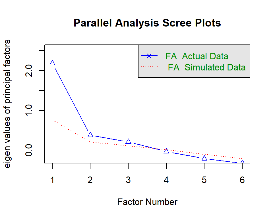
fa_aqi = fa(cor(df), nfactors = 3, fm = "pa", rotate = "varimax")
fa_aqi

Factor Analysis using method =  pa
Call: fa(r = cor(df), nfactors = 3, rotate = "varimax", fm = "pa")
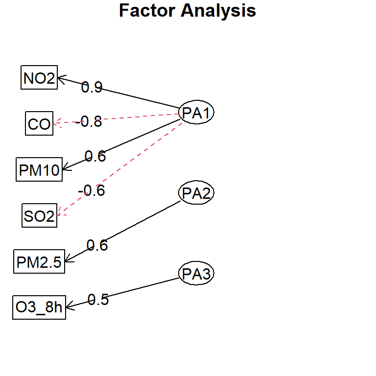
Standardized loadings (pattern matrix) based upon correlation matrix
        PA1  PA2   PA3   h2   u2 com
PM2.5 -0.06 0.63  0.03 0.40 0.60 1.0
PM10   0.61 0.47 -0.02 0.60 0.40 1.9
CO    -0.77 0.29  0.07 0.67 0.33 1.3
NO2    0.93 0.07  0.04 0.88 0.12 1.0
SO2   -0.61 0.01 -0.47 0.59 0.41 1.9
O3_8h -0.01 0.02  0.47 0.22 0.78 1.0

                       PA1  PA2  PA3
SS loadings           2.21 0.71 0.45
Proportion Var        0.37 0.12 0.07
Cumulative Var        0.37 0.49 0.56
Proportion Explained  0.66 0.21 0.13
Cumulative Proportion 0.66 0.87 1.00

Mean item complexity =  1.3
Test of the hypothesis that 3 factors are sufficient.

df null model =  15  with the objective function =  1.83
df of  the model are 0  and the objective function was  0 

The root mean square of the residuals (RMSR) is  0 
The df corrected root mean square of the residuals is  NA 

Fit based upon off diagonal values = 1
Measures of factor score adequacy             
                                                   PA1  PA2   PA3
Correlation of (regression) scores with factors   0.96 0.77  0.67
Multiple R square of scores with factors          0.91 0.60  0.44
Minimum correlation of possible factor scores     0.82 0.20 -0.11

返回结果首先给出的是标准化载荷矩阵，显示了三个因子对每个变量的标准化载荷。载荷大小表明因子对该变量的解释程度，其绝对值越接近1，解释程度越高，越接近0，解释程度越低，一般以0.5为临界值，PA1对PM10、CO、NO2和SO2的载荷绝对值都大于0.6，PA2仅对PM2.5的载荷绝对值大于0.6，PA3对SO2和O3_8h的载荷最大，但绝对值低于0.5。h2表示提取的因子对每个变量的解释程度，本例中三个因子对NO2的解释程度最高，而u2=1-h2，意义与h2相反。com是霍夫曼复杂度指数，反映原始变量受几个因子支配，本例中，对于PM10和SO2变量，都受两个因子的支配。

接下来的矩阵给出了三个因子的载荷平方和(SS Loadings)、所解释的方差(Proportion Var)、累积所解释的方差(Cumulative Var)、方差解释比例(Proportion Explained)和累积方差解释比例(Cumulative Proportion)。结果表明，三个因子所解释的累积方差只有0.56，其中PA1占比最大，为66%。

假设检验结果表明三个因子足以解释这些变量。

返回结果还包括因子得分充分性的测度，如相关性、R2、最小相关系数等。

利用fa.diagram()函数可以绘制出原始变量与公共因子之间的支配关系：

fa.diagram(fa_aqi)

由图 4.14 可见，前四个变量受第一个公共因子支配(红色表示载荷为负数)，PM2.5受第二个公共因子支配，O3_8h受第三个公共因子支配。在此基础上，可以尝试探究这三个公共因子的实际意义，PA1支配的4种污染物主要来自燃料燃烧、工业生产、机动车尾气排放等，可理解为初次污染物影响因子。PM2.5是PM10的组成部分，既有一次来源又有二次来源，还包括外源输入，因此PA2可能是综合的细颗粒物影响因子(PM10在PA2上的载荷为0.47)。O3是光化学反应产生的二次污染物，因此PA3可理解为二次污染物影响因子。

因子分子主要目的在于探究支配或影响原始变量的公共因子结构，而PCA方法则非常注重主成分的得分，以克服多变量多重共线性，用于建立定量模型。如果需要计算公共因子的得分，可以利用psych包中的facotr.scores()函数来计算，但计算结果因不同估计方法而不具有唯一性，而PCA中主成分的得分是唯一的。

fs = factor.scores(df, fa_aqi, method = "Thurstone")

输入fs$scores即可浏览原始数据集中每个观测的公共因子变量的得分。

结构方程模型是一种建立、估计和检验研究系统中多变量间因果关系的模型方法，利用图形化模型来展示研究系统中变量间的因果网络关系，可以替代多元回归、因子分析、协方差分析等方法，已经成为多元数据分析的重要工具，并在地学、生态学、环境科学与工程、医学、社会学、经济学等领域中应用十分广泛。如果需要执行SEM分析，可安装lavaan包，并在https://lavaan.ugent.be/网站学习该包的使用。

练习 4.6 (1)安装pls工具包，导入该包中内置的gasoline数据集，该数据集包括60个汽油样品的近红外光谱数据(NIR矩阵)。NIR矩阵的401列对应401个波长(从900nm到1700nm间隔2nm一个波长)的漫反射系数，octane为对应的辛烷值(octane)。对NIR矩阵进行主成分分析，并对前2个主成分进行可视化；然后以octane为因变量，以前2个主成分为自变量建立线性回归模型，并进行综合检验。
(2)基于内置数据集mtcars，执行因子分析；绘制前2个因子的载荷散点图，并标注对应的变量。

4.5 聚类分析和判别分析

聚类分析和判别分析都属于分类研究方法。前者是在类型未知情况下，利用样品(观测)或变量间的相似性，对样品或变量进行分类(一般称之为簇)；后者是在类型已知情况下，利用样品的特征(变量)值按选定的判定规则进行归类。按照机器学习方法的分类方法，聚类分析属于无监督学习，而判别分析属于有监督学习，前者主要用于特征降维，后者主要用于分类任务。

4.5.1 聚类分析

聚类分析也分为R型和Q型，前者对变量进行聚类，后者对样品进行聚类。通常，将聚集在一起的观测集合称之为一个簇(cluster)。聚类分析方法有很多种，包括基于划分的聚类(如k-means法等)、基于层次的聚类(如AGNES法等)、基于密度的聚类(如DBSACN法等)、基于网格或图的聚类(如STING法等)和基于模型的聚类(如EM法、SOM神经网络等)。聚类分析的目标就是使簇内相似度最高，簇间相似度最低。

聚类分析中相似度的测度有很多，例如欧氏距离、明氏距离(欧式距离的推广)、曼哈顿距离、马氏距离、切比雪夫距离、海明距离、余弦相似度、杰卡德相似系数(也称杰卡德指数)、杰卡德距离(杰卡德相似系数的补集，即与杰卡德相似系数之和为1)等。根据这些相似度的计算方法，可以编写相应的R语言聚类分析函数。

R语言已经预置了kmeas()和hclust()两个函数，分别用于执行k-means聚类和层次聚类(也称系统聚类)，此外，R包cluster、mclust、flexclust、fpc等还提供了更多类型的聚类分析方法。下面以R内置的iris数据集为例，利用cluster和factoextra包来演示Q型聚类分析。

例 4.51 对iris数据集进行聚类分析。

library(tidyverse)
library(factoextra)
library(cluster)
df = iris %>% dplyr::select(1:4)

先对各变量的观测值进行数值标准化：

dfs = scale(df)

接着用get_clust_tendency()函数对聚类趋势进行评估：

ct = get_clust_tendency(dfs, 50)

返回的结果为Hopkins统计量，该统计量的值越接近1，表明数据集的可聚类性越高，一般要求大于0.5。

ct$hopkins_stat

[1] 0.7997314

下面用eclust()函数进行聚类分析。该函数先估计最佳聚类簇数，然后根据最佳聚类簇数和指定的聚类算法进行聚类。如果指定了参数k的值，则无需估计最佳聚类簇数，直接根据k的值进行聚类分析。实际上，eclust()估计最佳聚类簇数是调用cluster包中的clusGap()函数，该函数通过自举抽样方法计算从1到指定最大簇数(参数k.max，默认值为10)的Gap统计量来确定最佳聚类簇数。

# 在1~6之间确定最佳簇数，并调用kmeans()函数执行聚类分析
kmc = eclust(df, FUNcluster = "kmeans", k.max = 6, nboot = 200, 
             seed = 2022, graph = FALSE)
kmc$gap_stat

Clustering Gap statistic ["clusGap"] from call:
cluster::clusGap(x = x, FUNcluster = fun_clust, K.max = k.max, B = nboot, verbose = verbose)
B=200 simulated reference sets, k = 1..6; spaceH0="scaledPCA"
 --> Number of clusters (method 'firstSEmax', SE.factor=1): 3
         logW   E.logW        gap     SE.sim
[1,] 4.551642 4.639505 0.08786357 0.02798343
[2,] 3.808397 4.190886 0.38248862 0.02328599
[3,] 3.519407 4.011100 0.49169324 0.02410995
[4,] 3.446685 3.917451 0.47076570 0.02519009
[5,] 3.301023 3.836240 0.53521663 0.02487646
[6,] 3.248167 3.760672 0.51250510 0.02451569

计算结果建议最佳簇数为3，这与iris数据集中的实际分类一致。下面用factoextra包中的fviz_gap_stat()可视化最佳聚类簇数估计的结果，如图 4.15 所示：

fviz_gap_stat(kmc$gap_stat)

接着使用fviz_cluster()对样品聚类结果进行可视化，结果如图 4.16 所示：

fviz_cluster(kmc, df)

已知iris中1-50、51-100以及101-150号样品分别归属为setosa、versicolor和virginica，查看哪些样品的聚类结果出现了偏差可以输入view(as_tibble(kmc$cluster))。

聚类结果有效性的评价方法分为外部评价法和内部评价法。外部评价法用于类别已知的数据集，包括纯度(Purity)、标准化互信息(Normalized Mutual Information)、兰德指数(Rand Index)、F值(F-score)等。内部评价法用于类别未知的数据集，同时考虑簇内和簇间相似度的评价指标有轮廓系数(Silhouette Coefficient)、CH指数(Calinski-Harabaz Index)、DB指数(Davies-Bouldin Index)、DV指数(Dunn Validity Index)等。这里只介绍轮廓系数的计算及其在R中的实现。对于某个样品，令a是其与同簇中其他样品的平均距离，b是与其距离最近的不同簇中样品的平均距离，则该样品的轮廓系数为

s=\frac{b-a}{\text{max}⁡(a,b)} \tag{4.32}

对于样品集合，其轮廓系数是所有样品轮廓系数的平均值。轮廓系数取值范围为[-1, 1]，取值越接近1表明聚类效果越好，越接近-1表明聚类效果越差。

cluster包中silhouette()函数用于计算轮廓系数：

sil = silhouette(kmc$cluster, dist(dfs))

该函数返回以个n×3的矩阵(n为集合中样品总数)，给出每个样品所在的簇(列名为cluster)、最近的族(列名为neighbor)和轮廓系数(列名为sil_width)。

下面用fviz_silhouette()对轮廓系数进行可视化：

fviz_silhouette(sil)

  cluster size ave.sil.width
1       1   38          0.36
2       2   62          0.34
3       3   50          0.64

图 4.17 显示簇3轮廓系数最大，簇1和簇2都较低，而且出现了负值。下面来查看负值对应的样品号：

sil %>% as_tibble() %>% 
  mutate(row_ID = rownames(.)) %>% 
  filter(sil_width < 0)

# A tibble: 6 × 4
  cluster neighbor sil_width row_ID
    <dbl>    <dbl>     <dbl> <chr> 
1       2        1  -0.226   51    
2       2        1  -0.0669  57    
3       2        1  -0.00928 66    
4       2        1  -0.124   87    
5       1        2  -0.0123  112   
6       1        2  -0.342   135

接下来采用层次聚类法(调用hclust()函数)进行聚类。为了与上面的k-means聚类结果进行公平的比较，最佳聚类簇数保持一致，即k = 3。但要注意，如果基于hclust()函数进行自举抽样估计，推荐聚类簇数为k = 5，按此簇数进行聚类，结果可以发现，簇数的增加主要是在原簇1和簇2下进行了细分。

hc = eclust(df, FUNcluster = "hclust", k = 3, graph = F)

对样品聚类结果进行可视化，结果如图 4.18 所示：

fviz_cluster(hc, df, labelsize = 7, pointsize = 1, ggtheme = theme_bw())

计算轮廓系数并可视化，结果如图 4.19 所示：

sil_hc = silhouette(hc$cluster, dist(dfs))
#rownames(sil_hc) = iris$Species
fviz_silhouette(sil_hc)

  cluster size ave.sil.width
1       1   50          0.64
2       2   64          0.34
3       3   36          0.39

比较图 4.16 与图 4.18 ，可见k-means聚类和层次聚类的结果在簇1和簇2(层次聚类结果对应簇3和簇2)有差异，层次聚类结果略有改善。图 4.19 显示层次聚类方法的平均轮廓系数为0.45，略高于k-means聚类方法的0.44，且仍有个别样品的轮廓系数为负值，下面来查看这些样品：

sil_hc %>% as_tibble() %>% 
  mutate(row_ID = rownames(.)) %>% 
  filter(sil_width < 0)

# A tibble: 5 × 4
  cluster neighbor sil_width row_ID
    <dbl>    <dbl>     <dbl> <chr> 
1       2        3   -0.205  51    
2       2        3   -0.222  53    
3       2        3   -0.0557 57    
4       2        3   -0.0955 87    
5       3        2   -0.0326 112

结果显示只有5个样品的轮廓系数为负值，而k-means聚类结果则有6个样品为负值。

传统的k-means聚类算法不能用于非凸数据集，而且对噪声和离群点非常敏感，大数据集的聚类结果容易陷入局部最优。kernlab包提供的基于核函数的k均值算法(kkmeans()函数)能够克服经典k均值算法的缺点。此外，fpc包提供了很多灵活的聚类算法，其中就包括基于密度的聚类算法(dbscan()函数)，同时也提供了聚类簇数估计、聚类结果有效性评估以及可视化的功能。mclust包提供了基于模型的聚类分析方法(还具有分类和密度估计功能)，通过期望最大化(EM)算法拟合高斯有限混合模型。pvclust包提供了基于多尺度自举抽样方法来评估层次聚类算法的不确定性。

4.5.2 判别分析

判别分析是在分类确定的条件下，根据样品的各种特征值(亦称判别变量)判定其类别归属问题的一种多元统计分析方法。判别分析需要先通过所谓的“训练样本”建立判别规则，然后利用判别规则对新的样品进行分类。判别分析主要分为距离判别分析、Fisher判别分析和Bayes判别分析三大类。距离判别分析根据欧氏距离、马氏距离等测度建立判别规则。Fisher判别分析则是一种基于投影的方法，将高维数据投影到一维空间，并使得投影后的类间方差最大、类内方差最小，从而实现分类，包括线性判别分析(LDA)、二次判别分析(QDA)等。其中LDA假设每个类别的数据服从多元正态分布，且各类别的协方差矩阵相同，判别函数是线性的；而QDA则允许各类别的协方差矩阵不同，判别函数是非线性二次函数。Bayes判别分析(BDA)基于贝叶斯定理，利用先验概率和似然函数来计算后验概率，然后将样品划分到后验概率最大的类别中。

R中MASS包中的lda()和qda()函数分别用于执行LDA和QDA。mda包中的mda()函数用于混合判别分析(MDA)，该方法仍然假设各类别的协方差矩阵相同，但每个类别被假设为子类的高斯混合)；该包中的fda()函数则用于弹性判别分析(FDA)，这是LDA的一种扩展，用于处理非线性关系或多变量非正态分布。klaR包中的rda()函数用于正则化判别分析(RDA)，对于存在多重共线性的数据集更稳健。klaR包中的NaiveBayes()函数和e1071包中的naiveBayes()函数都可用于执行BDA。距离判别分析可用kknn包中的kknn()函数，该函数执行k最近邻算法(k-Nearest Neighbor)，这也是一种原理简单但高效的机器学习算法。

下面演示LDA和BDA在内置数据集iris上的应用。

例 4.52 对iris数据集应用LDA和BDA。

先加载相关的R包：

library(MASS)
library(klaR)
library(dplyr)

载入iris数据集：

df = iris

将数据集分割为训练集和测试集：

set.seed(2022)
dftr = df %>% group_by(Species) %>% sample_n(40) 
dfte = setdiff(df,dftr)

基于训练集建立LDA判别模型：

m_lda = lda(Species ~ ., data = dftr)

对预测集进行预测：

pre_lda = predict(m_lda, dfte)

比较实际分类和LDA模型分类结果：

(tbl_tr_lda = table(dftr$Species, predict(m_lda, dftr)$class))

            
             setosa versicolor virginica
  setosa         40          0         0
  versicolor      0         39         1
  virginica       0          0        40

训练集上，LDA方法将1个veriscolor类的样品错分为virginica类。

(tbl_te_lda = table(dfte$Species, pre_lda$class))

            
             setosa versicolor virginica
  setosa         10          0         0
  versicolor      0          9         1
  virginica       0          1         9

预测集上，LDA方法分别将versicolor和virginica类中的1个样品错分。

下面来计算LDA方法的判对率：

cat("训练判对率：", sum(diag(prop.table(tbl_tr_lda))))

训练判对率： 0.9916667

cat("\n")    # 换行

cat("预测判对率：", sum(diag(prop.table(tbl_te_lda))))

预测判对率： 0.9333333

接下来采用klaR包中NaiveBayes()函数进行BDA。基于训练集建立BDA模型：

m_bda = NaiveBayes(Species ~ ., data = dftr)

对预测集进行预测：

pre_bda = predict(m_bda, dfte)

比较实际分类和BDA模型分类结果：

(tbl_tr_bda = table(dftr$Species, predict(m_bda, dftr)$class))

            
             setosa versicolor virginica
  setosa         40          0         0
  versicolor      0         38         2
  virginica       0          3        37

在训练集上，与LDA相比，BDA错分了5个样品。

(tbl_te_bda = table(dfte$Species, pre_bda$class))

            
             setosa versicolor virginica
  setosa         10          0         0
  versicolor      0         10         0
  virginica       0          1         9

在预测集上，与LDA相比，Bayes判别分析只错分了virginica类别中的1个样品。下面来计算Bayes方法的判对率：

cat("训练判对率：", sum(diag(prop.table(tbl_tr_bda))))

训练判对率： 0.9583333

cat("\n")

cat("预测判对率：", sum(diag(prop.table(tbl_te_bda))))

预测判对率： 0.9666667

LDA模型可以通过plot()函数进行可视化，具体参考其帮助信息。klaR包中的partimat()函数可以基于指定的判别方法对数据集中所有判别变量的两两组合进行可视化，其中参数method可指定为”lda”、“qda”、“rpart”(决策树方法)、“naiveBayes”、“rda”、“sknn”(简单k最近邻方法)和”svmlight”(支持向量机方法，需要安装SVMlight软件)。

library(klaR)
partimat(Species ~ ., data = iris, method = "lda", main = "LDA")

partimat(Species ~ ., data = iris, method = "qda", main = "QDA")

partimat(Species ~ ., data = iris, method = "rda", main = "RDA")

library(klaR)
partimat(Species ~ ., data = iris, method = "naiveBayes", main = "BDA")

library(klaR)
partimat(Species ~ ., data = iris, method = "rpart", main = "RPART")

library(klaR)
partimat(Species ~ ., data = iris, method = "sknn", main = "KNN")

练习 4.7 (1)从https://archive.ics.uci.edu/dataset/109/wine下载数据，基于葡萄酒化学分析变量进行聚类分析，然后根据class变量评价聚类分析的结果。
(2)继续基于上述wine数据集，执行LDA和BDA。